Lab 9: Mapping

The purpose of this lab was to place our robot in an unknown environment, shown below, and have it create a map of this environment.

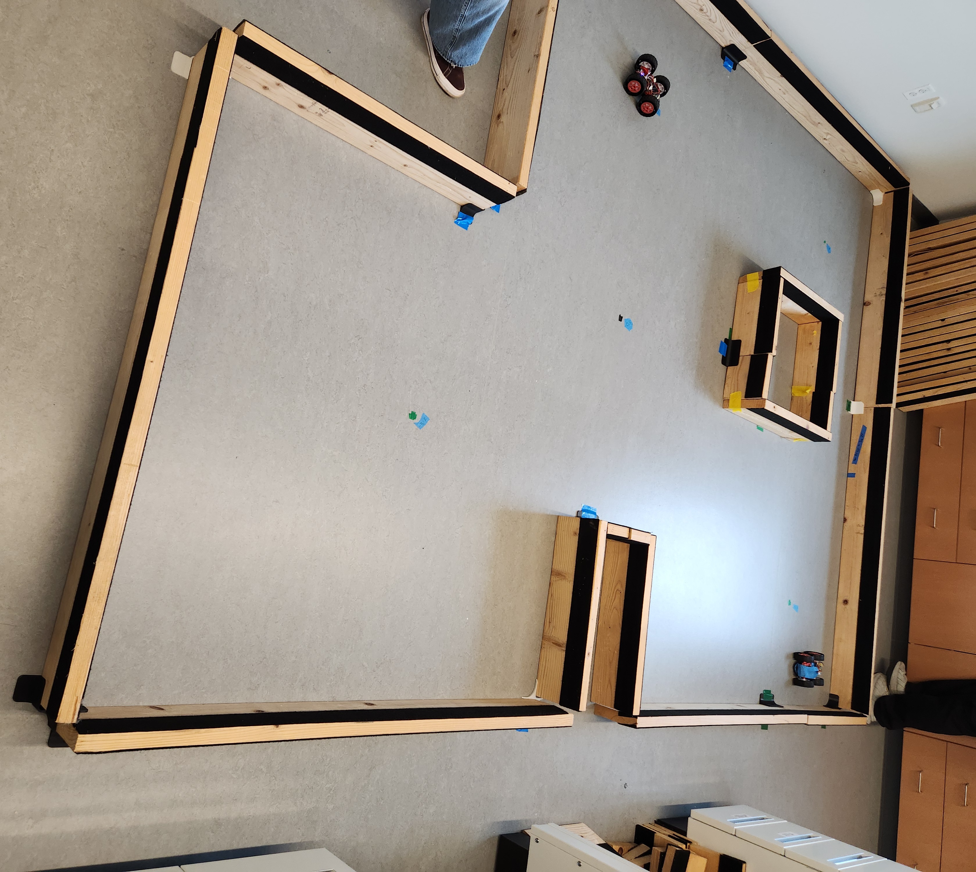
In order to map the world, the robot had to rotate at least 360° about certain points within the world without translating away from those points, collect many distance measurements, and then transform this data from the robot’s reference frame to that of the world’s.

Controlling the Robot’s Rotation

To control the robot’s orientation while rotating and taking measurements, I decided to use the PID controller I had already implemented for orientation control. I created a function mapping(), within which I keep track of the heading and how many rotations the car has completed in order to determine which angle to set the goal heading to next for the PID controller. The function is called upon receiving a DO_MAPPING command from my laptop, which also sets the flags angle_increment and number_of_rotations. These flags determine how many degrees the car jumps between calls to the PID controller, and how many full rotations the car should complete, respectively.

       case DO_MAPPING:
           success = robot_cmd.get_next_value(angle_increment);
           if (!success)
               return;
           success = robot_cmd.get_next_value(number_of_rotations);
           if (!success)
               return;
           internal_counter = 0; # Used to keep track of number of measurements
           disable_motors = 0; # allows motors to be ran
	    accumulated_angle = 0.0; # keeps track of how much the robot has rotated 
           mapping();
           disable_motors = 1; # doesn’t allow motors to be ran
           transmit_mapping_info(); # sends all data collected during mapping process
           break;

Within the mapping() function, a while loop tracks how many rotations have been completed by the robot. As long as the robot has completed less rotations than what was input, the car slowly rotates in increments of angle_increment degrees.

At each heading, the robot waits until it can collect distance data from the ToF sensor on the front of the robot. For this lab, I had to change the ToF sensors from short distance sensing mode to long distance sensing mode so that I could more accurately map the large distances within the world. The short distance mode’s maximum range of 1.3 m was just too small for this environment.

Once a measurement has been taken, the estimate of yaw is taken from the IMU via the DMP. With this angle, and with the previous angle of the car stored as a variable, I am able to check if the car has completed a full rotation by checking the signs of these values. Since I operate my system from -180° to 180°, one rotation occurs when the heading moves from a negative to positive value.

       angle = wrap_180(return_yaw_measurement(accumulated_angle));
       if ( (previous_angle < 0.0 ) && (angle >= 0.0) ){
           rotations = rotations + 1;
       }
       previous_angle = angle;

Then, mapping() populates the data of interest into their respective arrays. Names, the measured heading, the measured distance, and the time at which the current while loop iteration is running. This data will be sent to my laptop via Bluetooth upon the termination of the mapping() function, where it will be saved to CSV files.

After storing the data, I calculate the new goal angle based on the current heading and the angle_increment value. I have to ensure that this goal_angle is between 0° and 360°, which is the input range of my wrap_180() function.

       accumulated_angle = accumulated_angle + angle_increment;
       goal_angle = accumulated_angle + goal_angle_offset;
       if (goal_angle > 360.0){
           goal_angle_offset = goal_angle_offset - 360.0;
           goal_angle = accumulated_angle + goal_angle_offset;
       }

The desired heading is then set to goal_angle, and run_angular_pid() runs until the heading is achieved, at which time it sets heading_achieved to 1.

       while( !heading_achieved ) {
           run_angular_pid();
       }

Once the heading is achieved, this while loop is exited and heading_achieved is set back to 0. internal_counter is then incremented, and to slow the whole system down, I insert a delay for 1 second.

This continues until the number of desired rotations has been achieved.

Determining Reliability of Rotation and Measurement

I executed the above function at five separate locations in the world: (0, 0), (0, 3), (5,3), (5,-3), and (-3,-2). Importantly, those coordinates are in feet, not meters. For simplicity, I convert these to mm and name them Spot 4, Spot 1, Spot 3, Spot 5, and Spot 2, respectively.

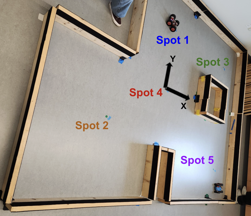
Before beginning the measurement taking process, I would orient the robot so that a heading of 0° corresponded to pointing directly into the +y direction of the world’s reference frame.

When using the data measurements, I had to determine how accurately my PID controller was able to achieve heading increments of 10° (~0.175 radians) throughout the entire rotation. To test this, I took measurements at Spot 4 for one rotation. This can partially be seen in the video below. Unfortunately, I started the video after the data collection had started, but the results of this data collection can be seen in the graph that follows the video.

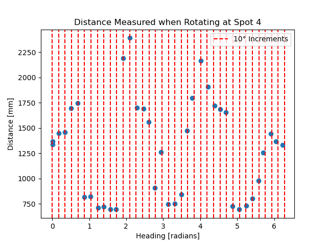
As it can be seen, the angles that the car believes that it is at seems to match pretty well with the desired heading for each measurement taken. Further analysis shows that the average error for this measurement was about -0.4°, with a variance of 1.46°, which can be visualized in the following graph.

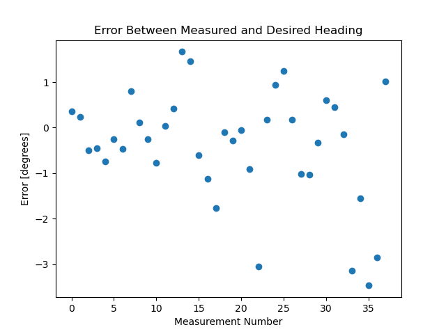
This error in angle seems relatively small with respect to the magnitude of a full rotation and implies that the robot behavior is reliable enough to trust when developing the map. However, this is important to keep in mind when thinking about how accurate the map is.

Additionally, I checked what the measured data looked like when the car rotated twice at Spot 5. Here, it can be seen that the measured data doesn’t exactly overlap, and the discrepancy is larger in areas that are farther away from the robot. Due to the fact that the robot is able to achieve the desired angle with relatively high accuracy, I think that this error may be mostly due to a slight translation of my robot as it rotated. This was not ideal behavior, but my robot would sometimes end up 100 mm, at a general maximum, from the point it started. This translation could have caused the ToF sensor to see different parts of the map as it made its second rotation, which could help to explain this discrepancy.

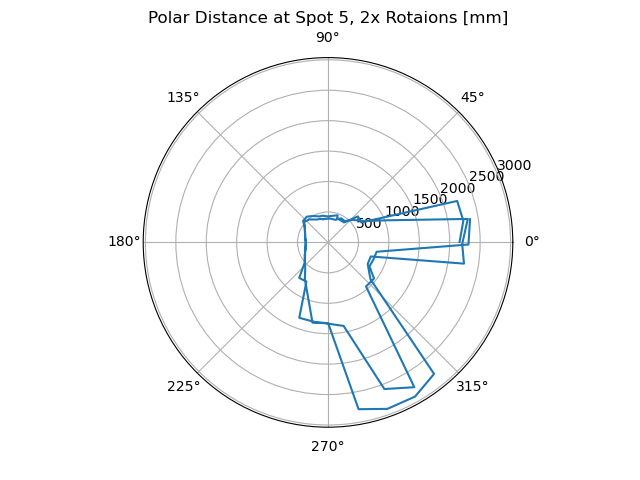
On average, when the robot is measuring an obstacle/wall, the error of the measured value compared to the true value seems to be smaller when measuring objects closer to the robot than farther away. It is hard to determine the exact error values because I don’t know at which point the car is making a measurement, but it looks like the error of the measurements of close obstacles seems to be on the order of ~50 mm at maximum. This error, however, increases the farther the robot tries to sense, resulting in measurements outside of the physical boundaries of the world. This behavior can be seen in the map graph shown in the next section.

This distance error, in addition to the heading error discussed earlier, could compound to create even more error when attempting to map a world, even one as simple as a 4x4 m room. The error would increase the farther the actual obstacle is from the robot because a small angular error has more effect farther away from the robot than it does close to the robot. In the 4x4 m example room, this map would lose accuracy in the corners. Our world is much more confident, so it is important to keep in mind these inaccuracies when completing the map making.

Map Making

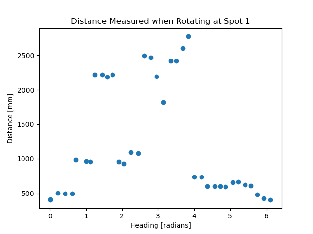
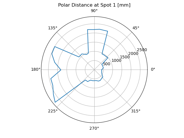
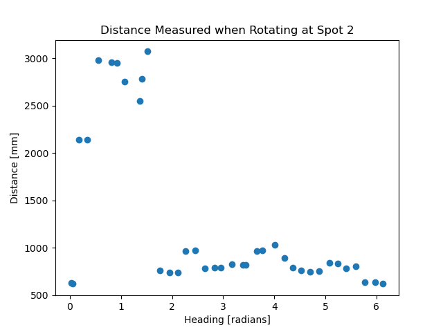
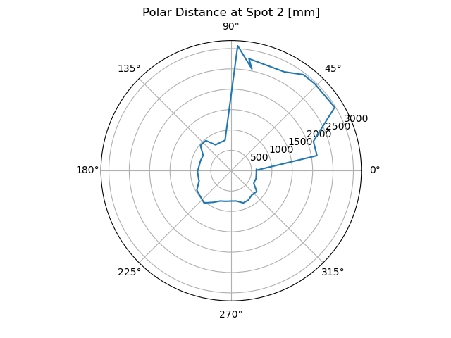
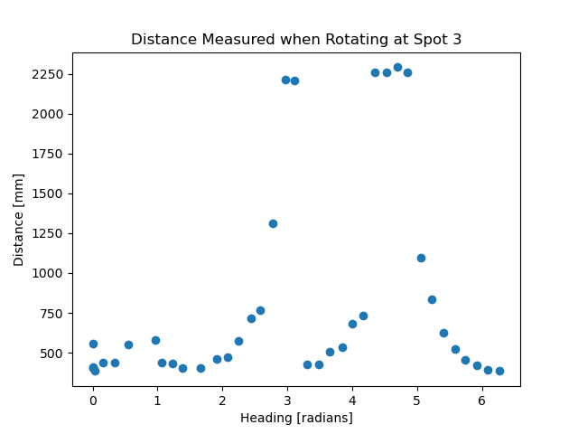
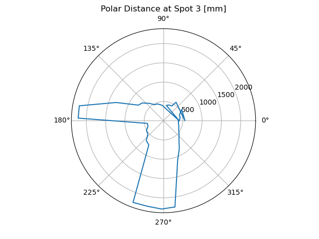
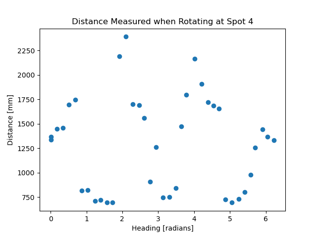
Here is the collected data from all of the spots:

Spot 1:

Spot 2:

Spot 3:

Spot 4:

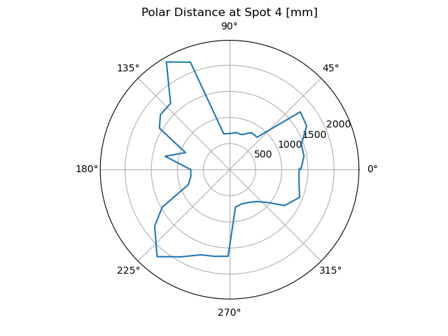
Spot 5:

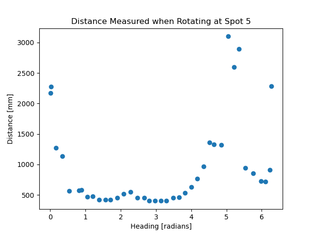
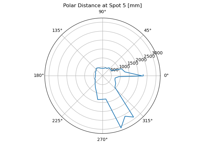
To convert this data, which is all centered about the robot, into a global map, I needed to use a transformation matrix to plot these data points in the world’s reference frame.

To do this, I created a transformation matrix that converted the data measured by the ToF sensor to the orientation of the center of the robot, and then a separate transformation matrix to convert the new coordinate to the global frame. Mathematically, this looks like:

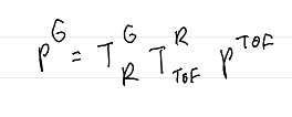
Here, P^ToF represents the measured point in the ToF’s reference frame, T^R_ToF represents the transformation from the ToF’s frame to the frame of the robot, T^G_R represents moving from the robot’s frame to the global frame of the world, and P^G represents the position of the measured distance in the world frame.

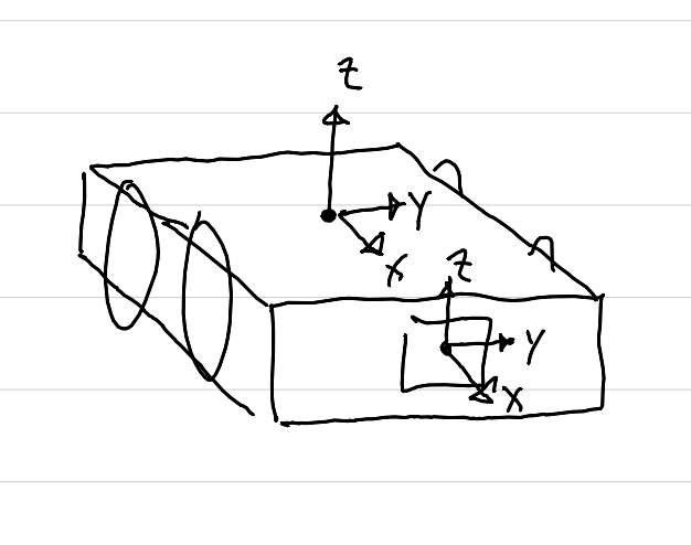
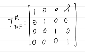
To determine T^R_ToF, I realized that if I create the orientation of the robot and the ToF to be the same, only translated along the robot’s x-axis by a distance L, then there would be no rotation. A visualization of this reference frame can be seen below, followed by the resulting transformation matrix:

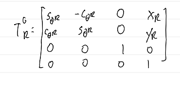
Moving from the robot’s frame of reference to the world’s frame was more difficult to think about. I realized that since I defined the robot’s x-axis to point in the world’s y-direction when the heading was 0, I was able to create a simple rotation matrix about the world’s z-axis. This resulted in a rotation where the sine of the robots heading times the component of the measurement in the robot’s x-axis minus cosine of the robot’s heading times the component of the measurement in the robot’s y-axis resulted in a vector pointing along the world’s x-axis. Similarly, the component of the measurement in the robot’s x-axis times cosine of the heading plus the component of the measurement in the robot’s y-axis times sine of the heading pointed along the global y-axis.

This created the rotation matrix between the robot’s frame and the world’s. The position of the robot in the world’s frame was simply equal to the coordinate of the Spot that it was at when taking the measurements, which I named x_R and y_R. This resulted in the following transformation matrix, where I am using short hand notation for sine and cosine, and theta_R is the robot’s heading:

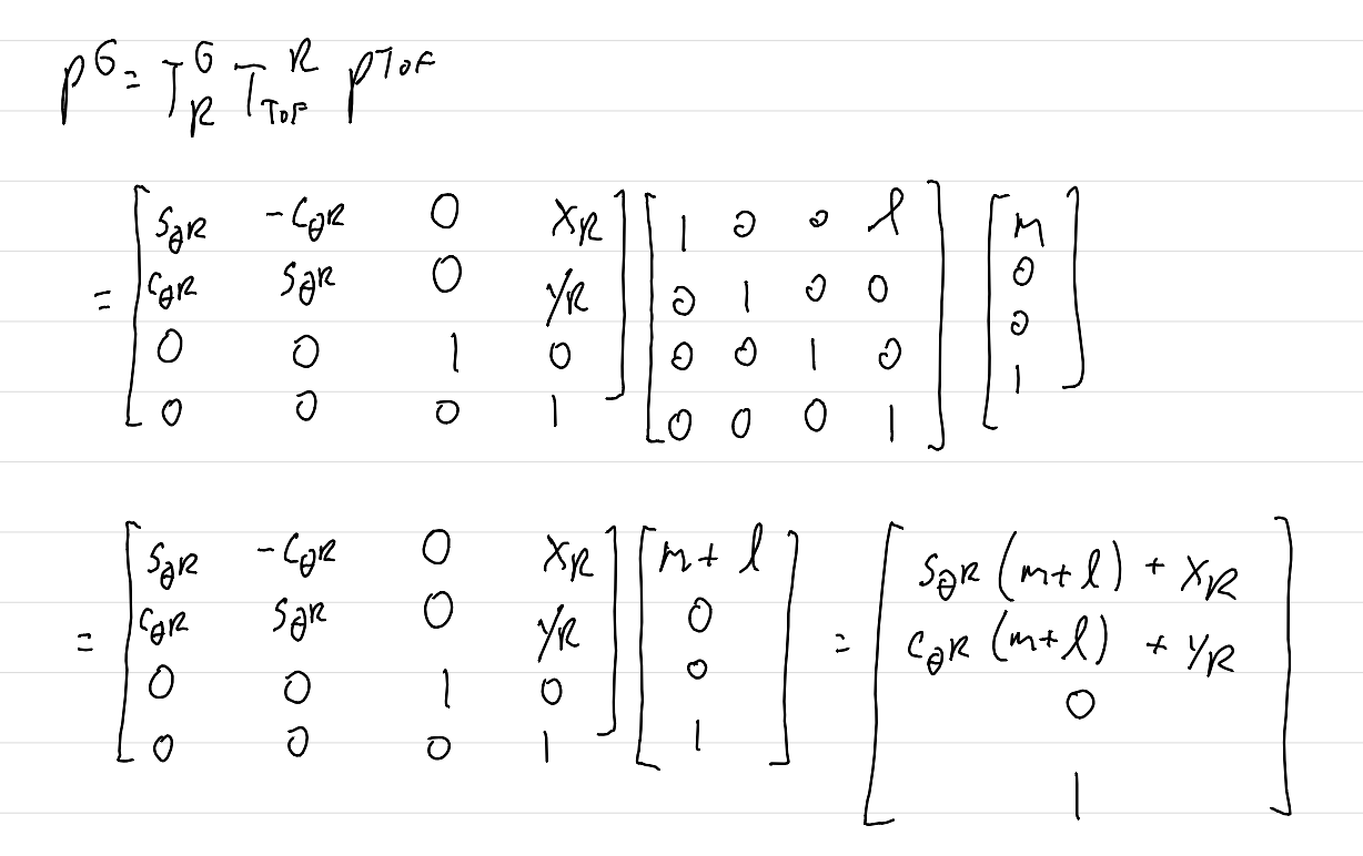
I then multiplied these matrices and the original position vector, where m is the ToF measurement:

I used this to create the following function in Python:

def transformation(measurement, x_R, y_R, theta_R):
    L = 82.55 # distance between ToF and center of robot
    # returns the x position in global frame, y position in global frame
    return (np.sin(theta_R)*(measurement+l) + x_R), (np.cos(theta_R)*(measurement+l) + y_R)

Then, I simply ran this function in a for loop with the distance and heading data, and output new coordinates in the global frame of reference. This resulted in the following map:

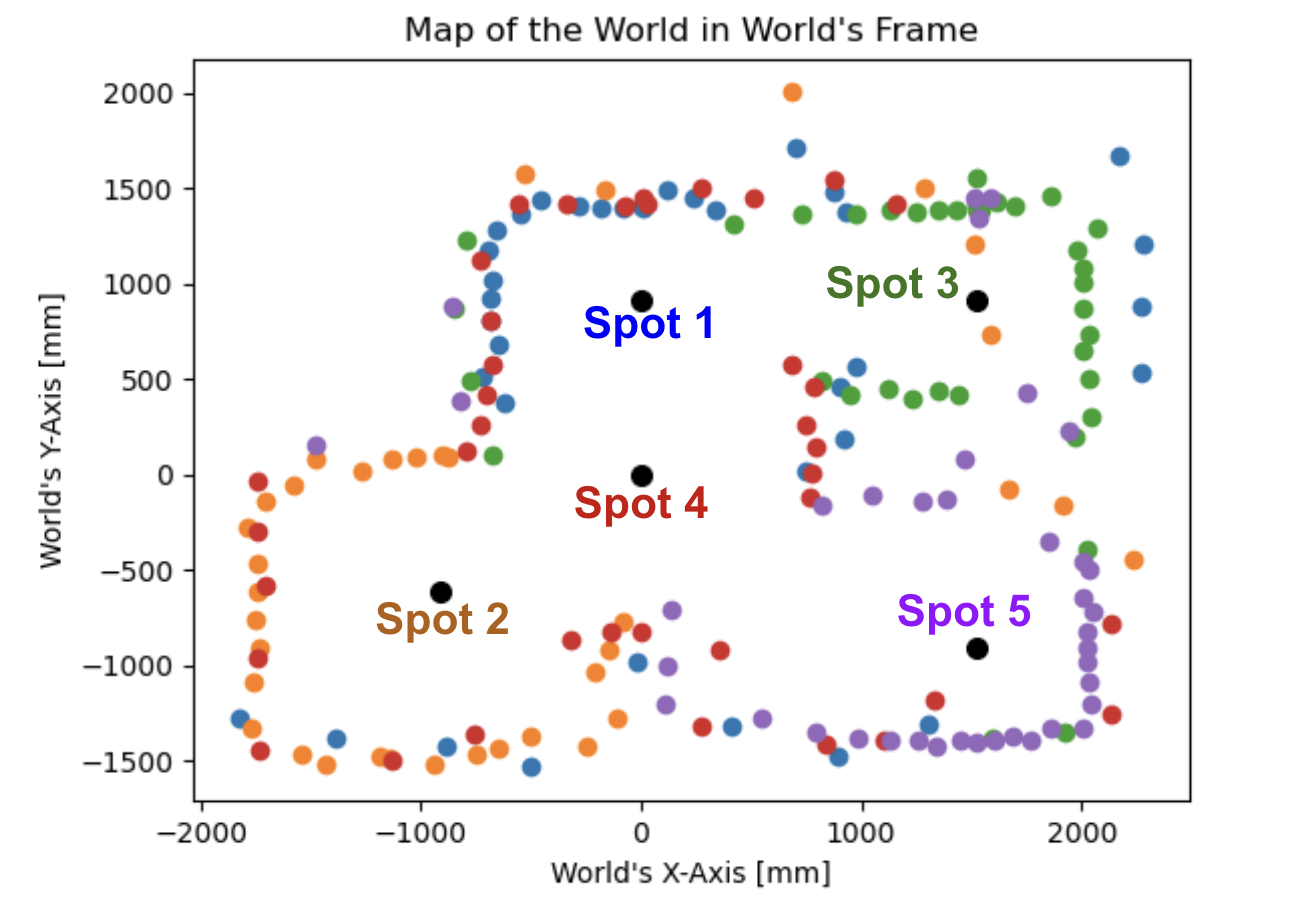
Taking into account the possible errors described earlier as well as clear outliers in the ToF data, I created the following world map:

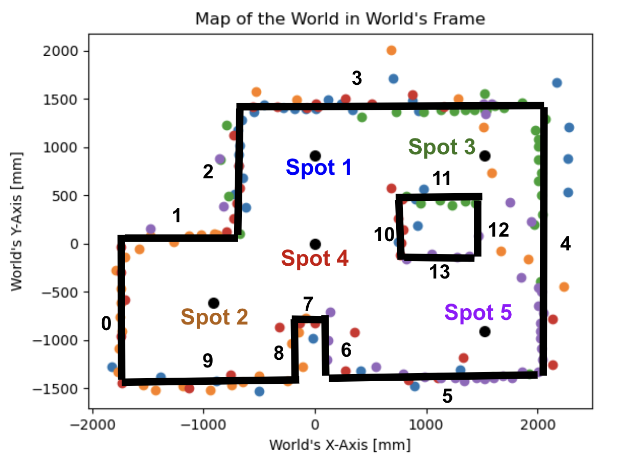
I input each line on this map into two separate lists, where the first list represents the beginning of a line and the second list represents the end of the line in mm. Similar indices in both lists correspond with their numbered line in the map shown above.

beginning_list = [[-1750, -1450],
                  [-1750, 50],
                  [-700, 50],
                  [-650, 1470],
                  [2070, 1470],
                  [2070, -1350],
                  [70, -1400],
                  [70, -750],
                  [-150, -750],
                  [-150, -1450],
                 ]

beginning_list = [[-1750, 50],
                  [-700, 50],
                  [-650, 1470],
                  [2070, 1470],
                  [2070, -1350],
                  [70, -1400],
                  [70, -750],
                  [-150, -750],
                  [-150, -1450],
                  [-1750, -1450],
                 ]