Lab 7: Kalman Filter

Introduction to Kalman Filters

Kalman filters provide a method to do state estimation stochastically. That is, instead of simply making a deterministic guess about a measurement like we did with the linear interpolation in Lab 5, a Kalman filter allows systems to predict their state and determine how confident that prediction is. This incorporates the uncertainty of any state dynamics and sensor measurements, allowing us to account for noise rather than pretend it doesn’t exist. This makes the Kalman filter an incredibly useful tool.

Kalman Filter Derivation

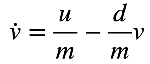
In order to implement a Kalman filter, we have to understand how our system evolves as a function of the state and of the input. In an ideal scenario, we have a linear system that can be described as:

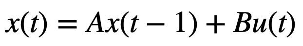
Here, the matrix A describes how the system evolves with no input and the matrix B represents how input into the system changes the state.

In the car’s system, the state could be represented as [position, velocity], and the change in the state would then be [velocity, acceleration]. With this choice of state, we can approximate our system as linear such that we have the following state evolution equation:

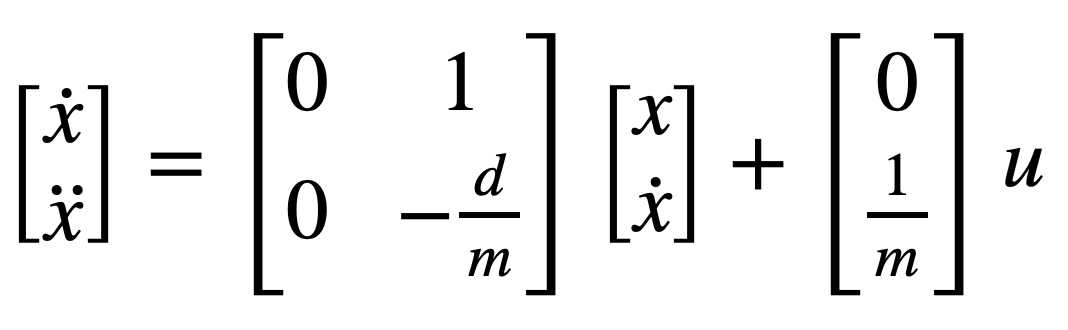
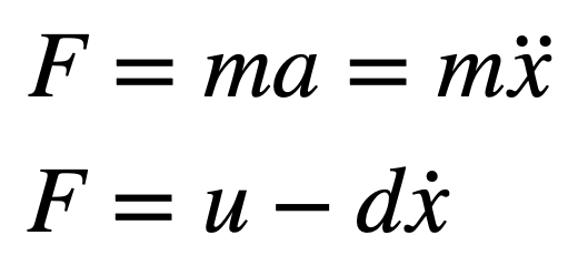
Here, the 2x2 matrix is A, and the 2x1 matrix is B. The only unknowns are d, a drag constant, and m, the inertial mass of the car. Luckily, these can be found by doing a force balance on the car and assuming that the PWM input, u, acts as a force on the car. From here, we can write:

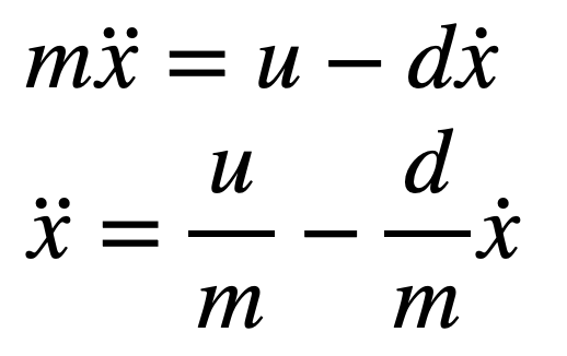
This allows us to solve for the acceleration and velocity in terms of u, m, and d:

In order to find d, we can provide a step response input to the car to cause it to drive forward, and then wait for the velocity to stop changing. At this steady state velocity, the acceleration would be zero and d would become equal to u divided by the steady state velocity. For simplicity, we can normalize the step response from whatever PWM input we choose to use. I decided to build my Kalman filter around a step response of a PWM input of 255 so that my car can perform well at high speeds.

I collected data about my car’s distance from a wall while driving towards it with a PWM input of 255. I took the average of four trials and plotted them below:

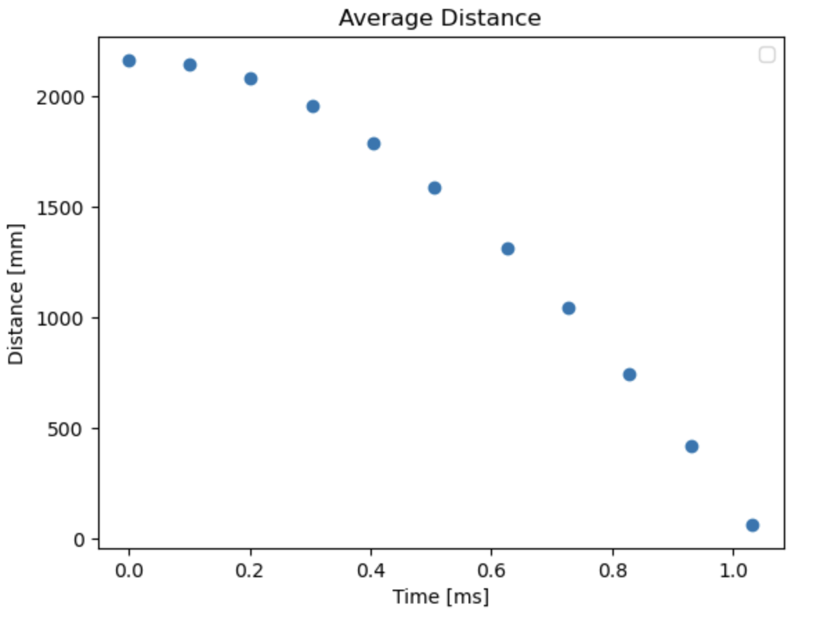
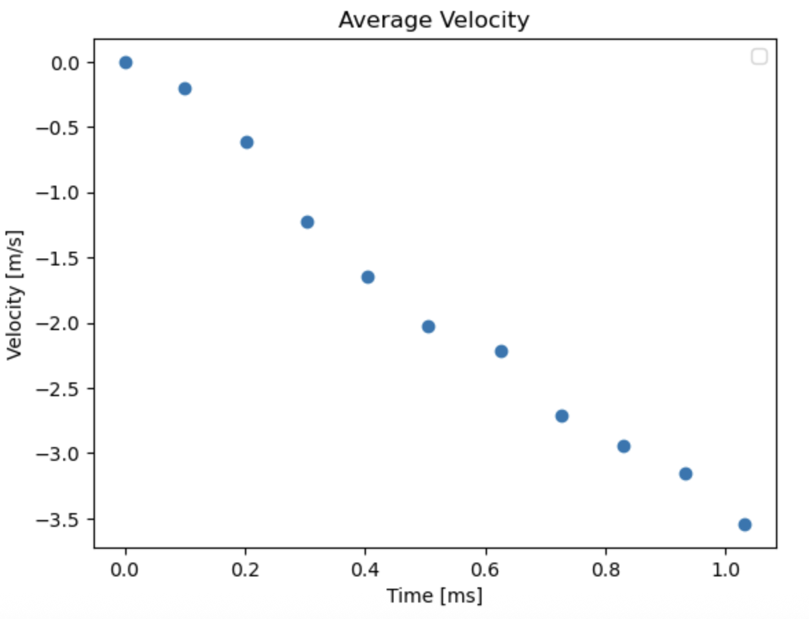
Unfortunately, the car wasn’t able to achieve a steady state velocity before hitting the wall, so I had to fit an exponentially decaying curve to the velocity data and approximate what the steady state velocity would be. I decided to leave out the first two velocity data points when fitting this curve because they corresponded to when my car was just starting to move and wasn’t accelerating too much.

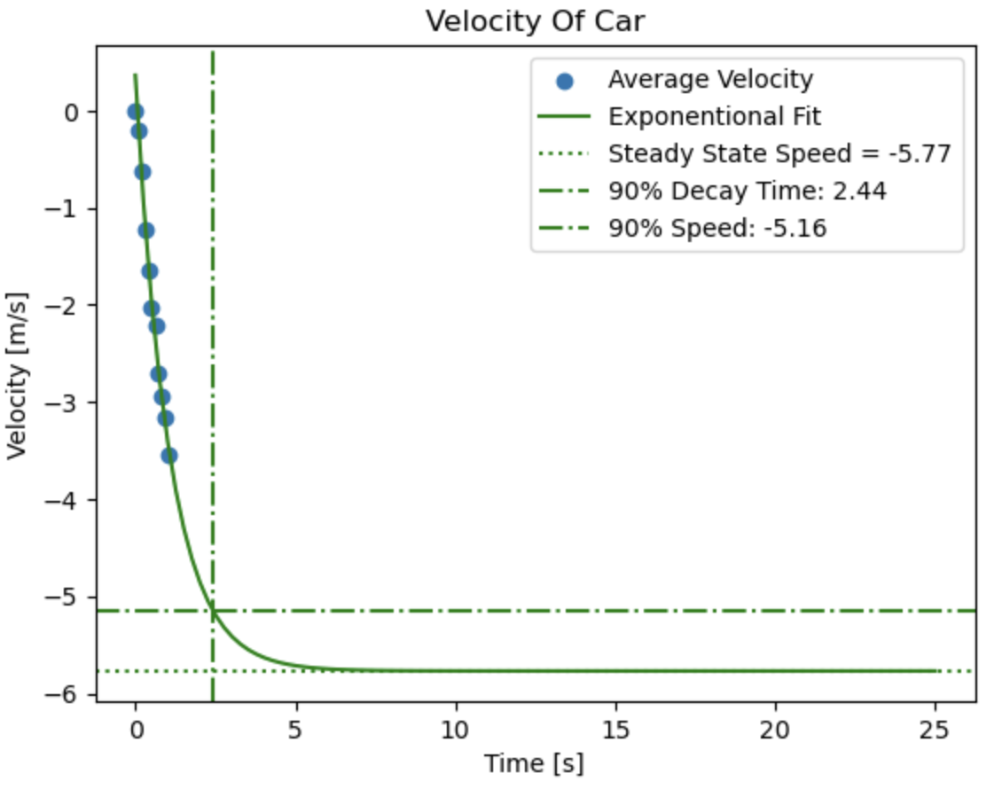
From this, I determined that d = 1/5769.887 = 0.0001733 [N*s/mm]. I found m by solving the first order Taylor expansion of:

Resulting in:

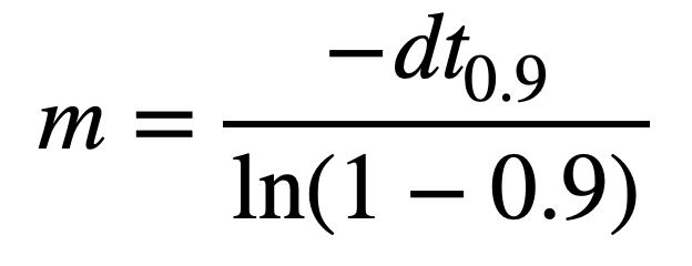
Here, t_0.9 is the 90% decay time, which is indicated in the graph of the exponential fit to be 2.43995 [s]. Therefore, m = 0.000183653 [N*s^2/mm].

Kalman Filter Tuning

With values for m and d, the A and B matrices could be built. These, however, correspond with continuous time, and this system operates in discrete time. To discretize these matrices, I computed the following for various dts.

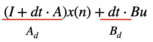
I first chose dt = 0.0909 as this corresponded with the sampling period of my ToF sensor. However, this was two slow of a dt to run the prediction step in between sensor readings, so I changed it to dt = 0.00909, which was about how fast my control loops ran at. It proved to be challenging to find an appropriate dt for my final version of the Kalman filter because my control loop wouldn’t maintain a constant frequency. To account for this, in my final implementation I calculate dt every iteration and compute Ad and Bd on the fly so that the estimation can adapt if the control loop slows down or speeds up.

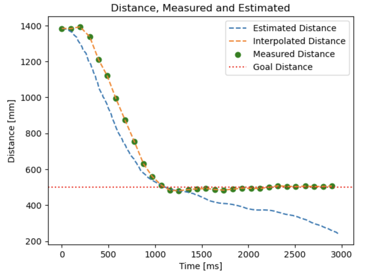
Additionally, a large part of tuning is determining what a good amount of measurement noise and process disturbance to give the filter is. When the measurement uncertainty was very high, the estimated distance didn’t correct itself if measurements were taken. To show this, I took data from Lab 5 and used it to characterize the behavior of the Kalman filter. Below, you can see how the Kalman filter doesn’t respond when the measurement noise is significantly higher than the process noise:

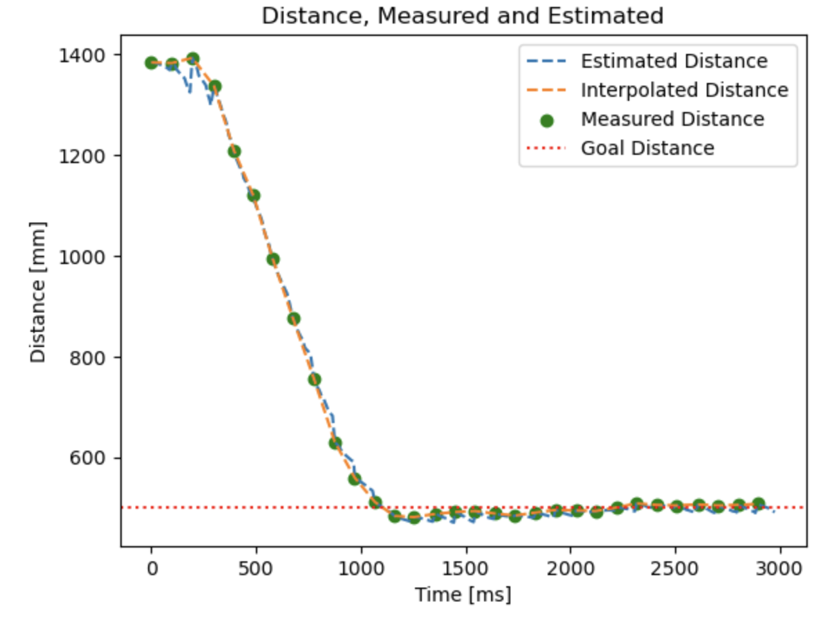
Conversely, if the process noise is very high relative to the measurement noise, the Kalman filter closely tracks the measurements as they come in:

Throughout the tuning process, I changed the values of these uncertainties a lot. Initially, I tried to reason about how uncertain the measurement noise would be based on previous data I had collected, and made rough order of magnitude estimates for the process noise. This was initially a measurement uncertainty of about 10, and a process uncertainty of about 20 for both the position and velocity. I then iteratively observed the Kalman filter’s response to the uncertainties, changed the uncertainties to either increase or decrease the significance of the measurements, and then observed the behavior again.

In order to visualize the behavior, I used these two functions to run the Kalman filter on the Lab 5 data:

def kf_predict(mu, sigma, u, s_u, Ad, Bd):
    mu_p = Ad.dot(mu) + Bd.dot(u) 
    sigma_p = Ad.dot(sigma.dot(Ad.transpose())) + s_u
    return mu_p,sigma_p

def kf_correct(mu, sigma, y, s_z, C):
    sigma_m = C.dot(sigma.dot(C.transpose())) + s_z
    kkf_gain = sigma.dot(C.transpose().dot(np.linalg.inv(sigma_m)))
    y_m = y-C.dot(mu)
    mu = mu + kkf_gain.dot(y_m)    
    sigma=(np.eye(2)-kkf_gain.dot(C)).dot(sigma)
    return mu,sigma

I called the predict and correct functions in a larger function that allowed me to quickly change the measurement and process uncertainties for efficient testing:

def run_filter(measurement_sigma, process_1_sigma_loop, process_2_sigma_loop, ToF_data, pwm_data, data_time, full_time):
    global PWM_step # = 255
    global C # control matrix of [[-1,0]]
    global Ad_sensor # the matrix Ad
    global Bd_sensor # the matrix Bd
    global initial_pos_uncertainty # initial uncertainty in position
    global initial_vel_uncertainty # initial uncertainty in velocity
    
    Sigma_z = np.array([[measurement_sigma**2]]) # uncertainty matrix of the measurement

    # uncertainty matrix of the process
    Sigma_u = np.array([[process_1_sigma_loop**2, 0], [0, process_2_sigma_loop**2]])

    # the initial state
    x = np.array([[-ToF_data[0]], [0]])

    # a list that will hold all of the states
    # generated by the filter
    estimated_distance = []
    estimated_distance.append(-x[0][0])

    # the initial uncertainty in the position and velocity
    Sigma = np.array([[initial_pos_uncertainty**2, 0], [0, initial_vel_uncertainty**2]])

    pwm_input = pwm_data[0]/PWM_step # scale the PWM signal appropriately

    j = 1
    for i in range(1, len(full_time)):

        # make the prediction every step
        x, Sigma = kf_predict(x, Sigma, pwm_input, Sigma_u, Ad_sensor, Bd_sensor)
        # make the correction if the sensor made a measurement at time full_time[i]
        if j < len(data_time) and abs(full_time[i] - data_time[j]) < 1e-4:
            pwm_input = pwm_data[j]/PWM_step # update the PWM signal
            # correct the prediction
            x, Sigma = kf_correct(x, Sigma, ToF_data[j], Sigma_z, C)
            j += 1
    
        estimated_distance.append(-x[0][0]) # add the prediction to the list

It is worthwhile noting that the PWM input u is equal to the true PWM input divided by 255, in order to account for the fact that this was set to unity when finding d and m.

Kalman Filter in Practice

I used a very similar structure on the Artemis to implement the Kalman filter:

void kf_predict(Matrix<1> input){
   state = Ad*state + Bd*input;
   Sigma = Ad*Sigma*~Ad + Sigma_u;
}


void kf_correct(Matrix<1> measurement){
   Sigma_m = C*Sigma*~C + Sigma_z;
   K_Gain = Sigma*~C*Inverse(Sigma_m);


   Matrix<1> y_m = measurement - C*state;
   state = state + K_Gain*y_m;
   Sigma = (Identity - K_Gain*C)*Sigma;
}

Whenever the controller ran, kf_predict was called to update the prediction and uncertainty of the state. If a new ToF reading was available, then I would also call kf_correct and use that reading to correct the prediction.

An issue that I ran into was that my filter would automatically move to wherever the measured distance was once a new data point was available, instead of slowly moving in that direction while also attempting to maintain its current course. This caused my filter to output distance values that changed quickly, which created a lot of large values in the derivative term of my PD controller. To counter this, I passed the derivative term through a stronger low pass filter, but this added some delay to the car’s reaction. This started a new PD tuning process, and I ended up selecting kp = 0.3 and kd = 0.15, both of which are higher than what I chose in Lab 5.

The following is an example of my car running the PD controller with a Kalman filter for estimating the distance from the wall instead of linear interpolation. For this run, I used a measurement uncertainty of 20, a position uncertainty of 10, and a velocity uncertainty of 15.

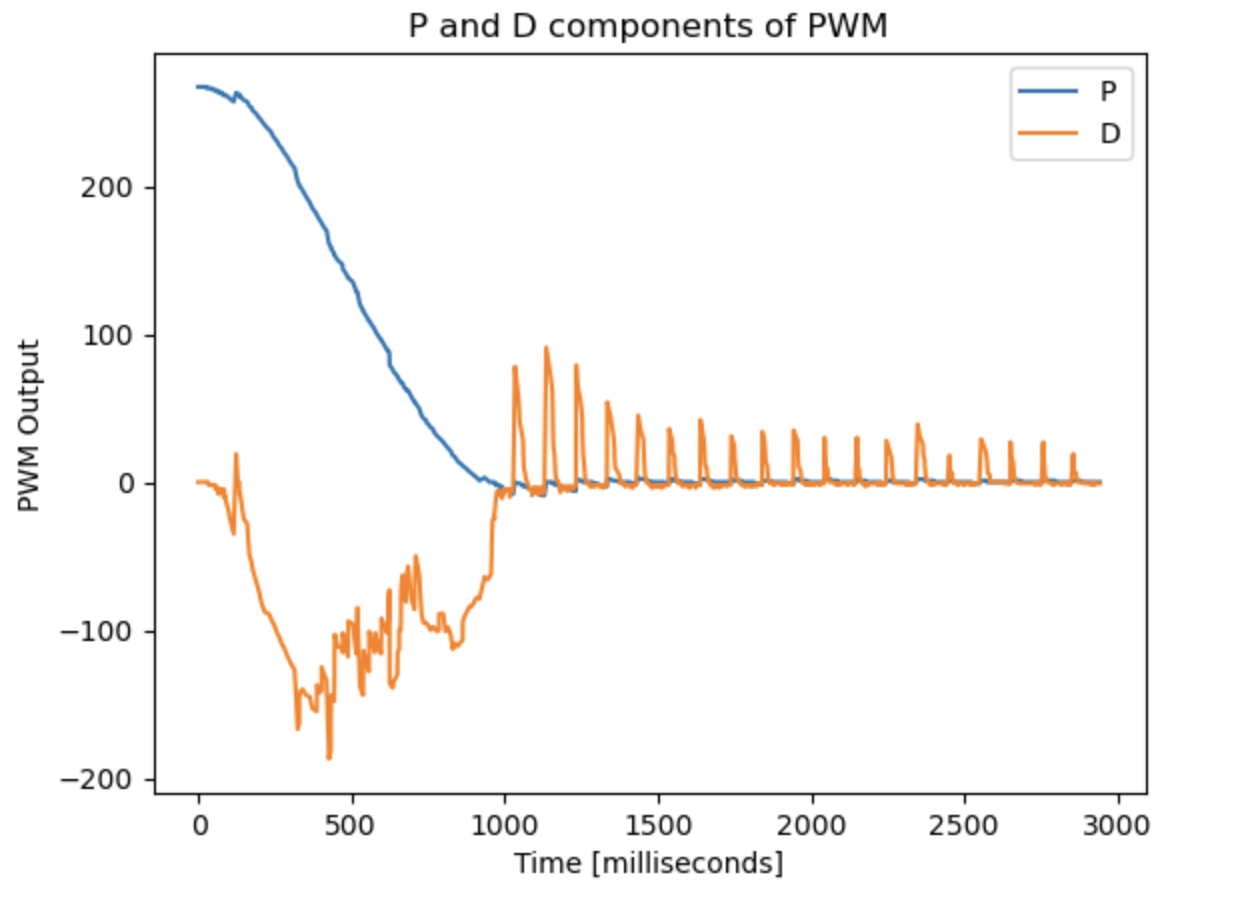
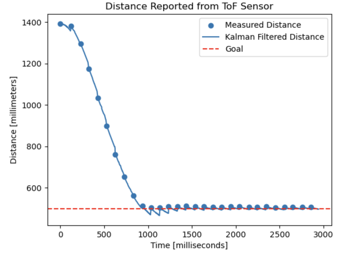
Interestingly, this implementation seemed to reach the setpoint quicker than the car did in Lab 5.

Acknowledgements

I referenced Stephan Wagner’s and Trevor Dales’ websites to compare the behavior of their Kalman filters with mine. I also used some of the lecture slide content for the images of Newtonian equations and Kalman filter equations in this report.