Lab 6: Orientation Control

Prelab

To control the orientation of the car, I had to implement a few more Bluetooth commands that the Artemis could use for the new PID controller.

I created a SET_ANG_PID_PARAMS command that set the values of kp, kd, and ki, even if the control loop was already running, allowing for fast experimentation. To start the orientation control loop, I sent the command START_ANGULAR_PID, and sending SEND_ANGULAR_PID_DATA triggered the transfer of any data collected back to my laptop for analysis.

Similarly to Lab 5, the code on the Artemis board would raise or lower different flags, depending on what commands were received. The void loop() then acted upon those flags. Below is some pseudocode describing my updated process in the void loop():

while there is a Bluetooth connection {


	Read any incoming Bluetooth commands
	Send any outgoing data over Bluetooth


	if the flag associated with running the distance PID loop
	is set high by the Bluetooth commands:
		run one iteration of the distance PID loop


	if the flag associated with sending the data collected while
	the distance PID loop ran is set high by the Bluetooth commands:
		send all relevant data


	if the flag associated with running the angular PID loop
	is set high by the Bluetooth commands:
		run one iteration of the angular PID loop


	if the flag associated with sending the data collected while
	the angular PID loop ran is set high by the Bluetooth commands:
		send all relevant data


	if the flag associated with cutting power to the
	motors is set high by the Bluetooth commands:
		stop the motors
}

Lab Tasks

PID Input Signal

In order to do control on the orientation of the robot, it was necessary to use the IMU to collect data of the yaw of the robot. Unfortunately, it isn’t possible to get yaw from the accelerometer alone, so the gyroscope is needed. In order to get yaw from the gyroscope, the angular velocity about the z-axis needs to be integrated. But, the gyroscope has a slight offset, or bias, from the true angular velocity. This causes the calculated yaw to drift from the true value by constantly integrating this error.

This issue could be somewhat avoided by subtracting the bias from any gyroscope readings. However, this may not work on longer time scales as the gyroscope bias can change.

Luckily, the IMU has a built-in alternative: a Digital Motion Processor, or DMP. The DMP uses the IMU’s accelerometer, gyroscope, and compass to perform motion processing algorithms on the IMU chip itself, all while running background calibrations. This data can be sent to the Artemis as a quaternion, which can then be transformed into Euler angles in order to get the yaw of the car.

With the DMP implemented, only two questions remain: can the gyroscope measure angular velocities that the car will rotate at, and can the DMP return orientation information fast enough? The gyroscope has a programmable range of measurements, and under DMP operation it can register angular velocities between ±2000 degrees per second. This is far beyond the rotational speed of our car.

Additionally, the DMP’s output data rate can be set when the IMU is initialized:

// Set the DMP output data rate (ODR): value = (DMP running rate / ODR ) - 1
// E.g. for a 5Hz ODR rate when DMP is running at 55Hz, value = (55/5) - 1 = 10.
success &= (myICM.setDMPODRrate(DMP_ODR_Reg_Quat6, 1) == ICM_20948_Stat_Ok);

I decided to set the output data rate to about 25 Hz as an initial test of the system. This did not bottleneck my control loop, which ran at about 190 Hz. I achieved this by holding the angle value constant whenever no new data was available. For a more adaptive interpolation method, I could have linearly extrapolated from the two most recent sensor readings like in Lab 5. I found that this was not necessary to achieve a low settling time, but this could be useful for future iterations.

Proportional Discussion

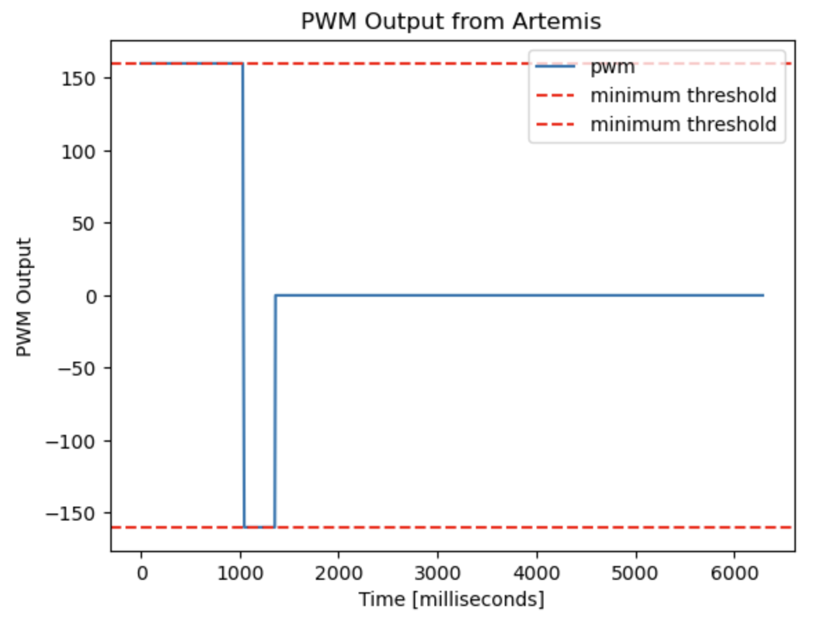
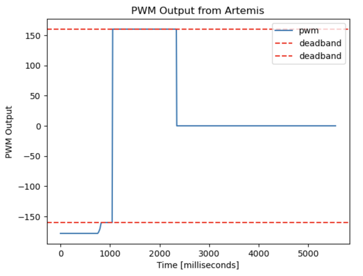
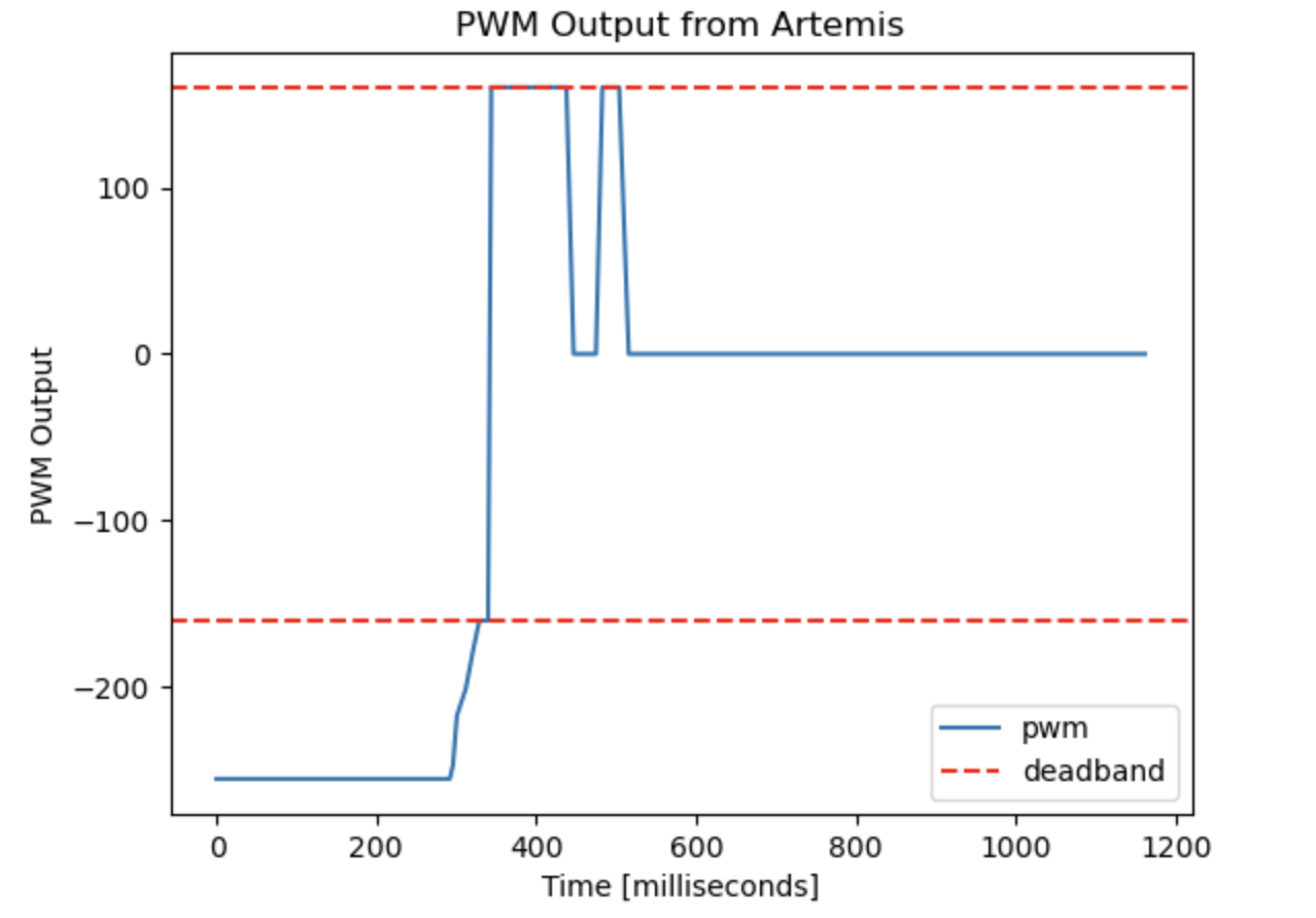
Recognizing that the maximum error I could get between the car’s current heading and the goal heading was 180°, I decided that I should first try a kp value of 1, as this would cause the maximum PWM signal to be 180. While this might seem large when compared to the PWM signals of Lab 5, this signal is being used for a completely different motion. Rotational motion requires more energy, and the deadband is significantly higher. Here, I set the deadband to 160, which is higher than what I found in Lab 3, but this allows for the car to move more smoothly.

In order to produce rotational movement, I set one set of wheels to drive forward with input PWM, and the other set of wheels to drive backward with the same PWM. If the PWM were to be negative, the direction of rotation would switch.

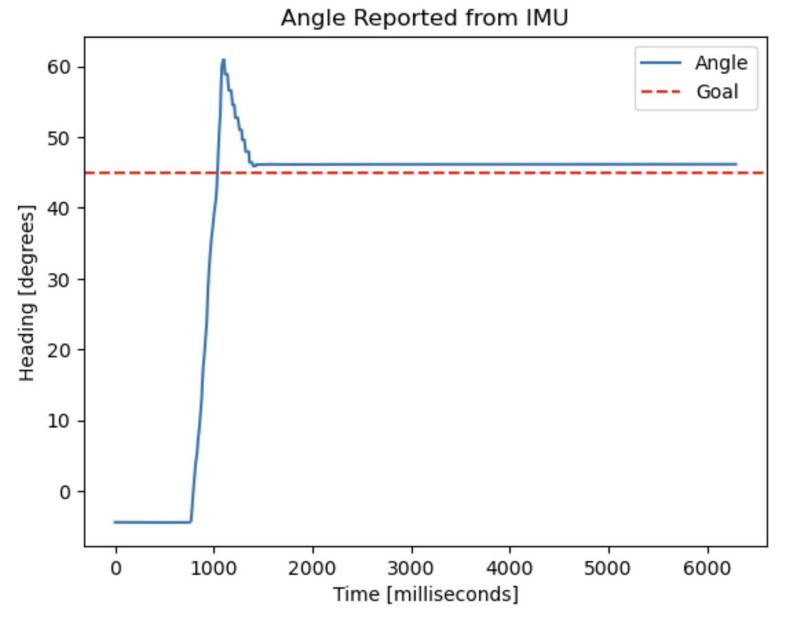
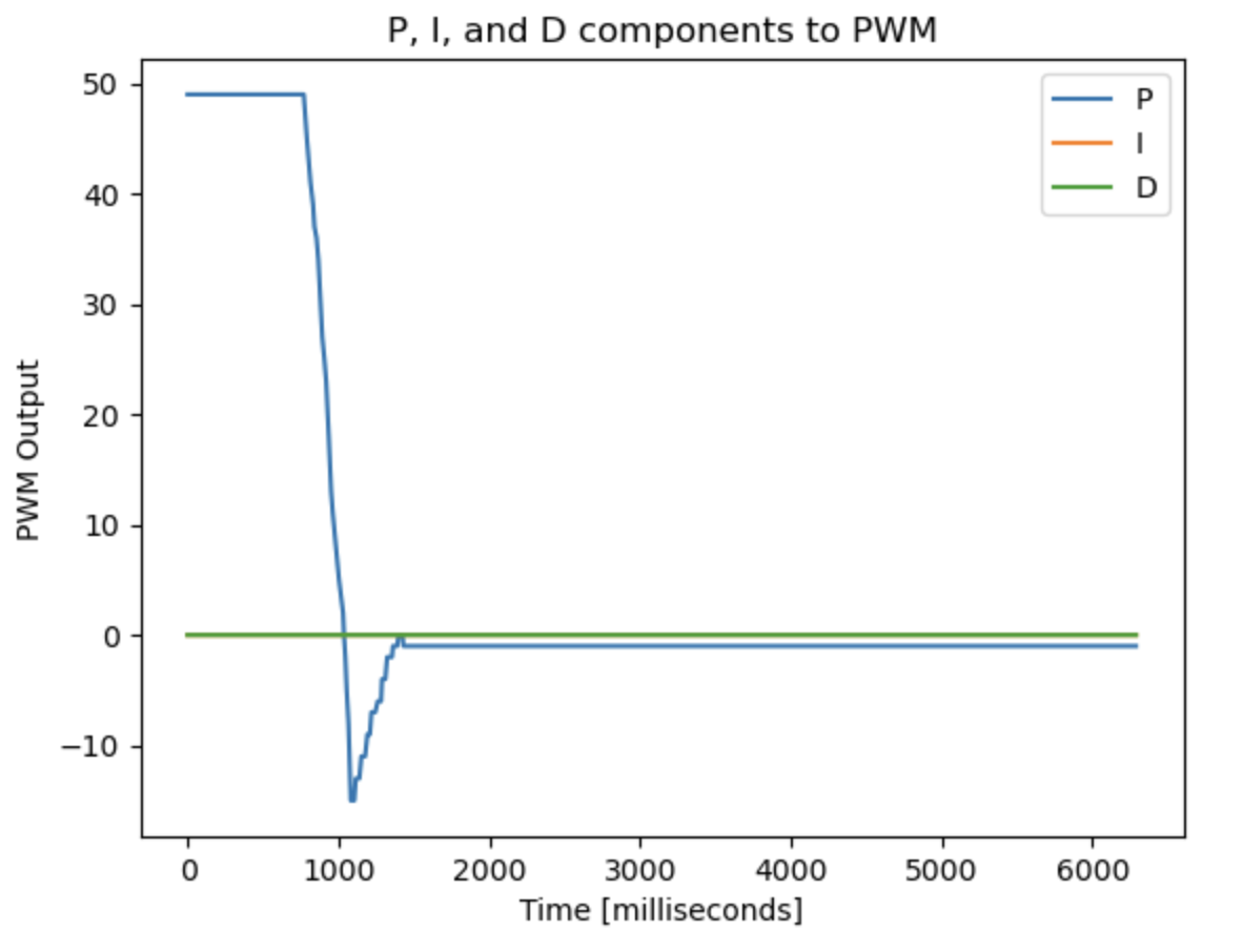
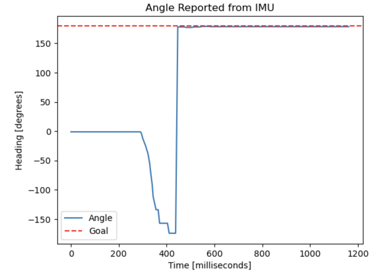
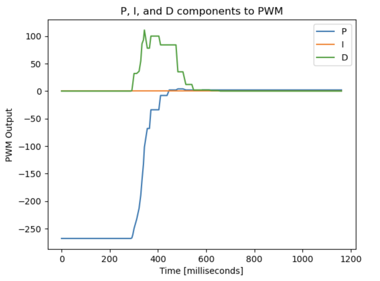
Using kp = 1.0 and kd = ki = 0.0 was a good start, but it resulted in a significant amount of overshoot. The following data was collected when the car was attempting to rotate 45° to the right.

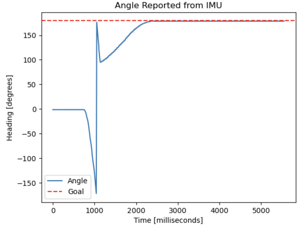
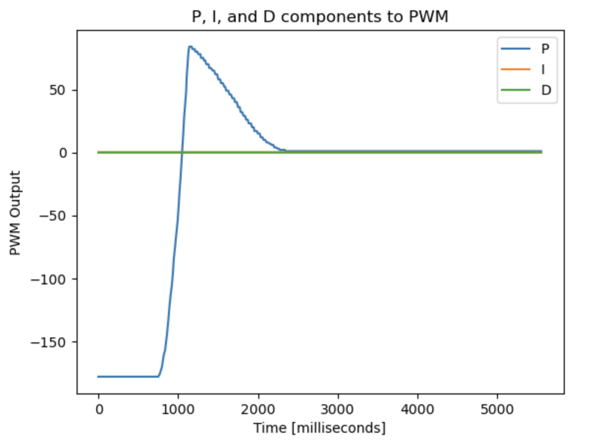
When the car attempted to rotate 180°, it overshoot even more.

Proportional and Derivative Discussion

To account for this overshoot, I needed to implement derivative control.

If I had not used the DMP, then calculating the derivative of the yaw would be straightforward since the gyroscope outputs the rate of change of yaw. However, with the DMP in place, I was not able to access the raw acceleration and gyroscope readings. I believe that this is due to the IMU prioritizing computation necessary to run the DMP and not basic readings.

Normally, I would not take the derivative of the integral of a noisy and biased signal, but the DMP’s internal sensor calibration causes its output to be more accurate than a filter that I might have created. Therefore, I thought it was appropriate to take a derivative of this data.

To prevent any derivative kick that might occur when initializing the system or changing the setpoint, I took the derivative of the heading instead of the error. This was a little bit challenging to implement since I decided to wrap my heading between [180,° -180°), but it just required a little bit more math. Additionally, I low-pass filtered the derivative of the heading in order to remove noise caused by the car jittering back and forth.

After many trials, I finally arrived at values of 1.5 and 0.03 for kp and kd were 1.5, respectively. This created a snappy response from the car with minimal overshoot.

The following video shows how the setpoint can be changed as the controller is running, as well as how the car can adapt to disturbances. Interestingly, the behavior of the car here is slightly less ideal than that in the previous video. This could be due to many factors, but I believe that it is because the motor battery didn’t have the exact same charge for the two demonstrations.

Integral Discussion

Similar to Lab 5, I found that the system did not encounter any steady state error, so I did not implement an integral portion in the control logic.