Lab 5: Linear PID Control and Linear Interpolation
Prelab
In order to efficiently tune the PID parameters, I had to restructure how the Artemis handles Bluetooth commands sent from my laptop. Originally, I sent a single command that set all of the values of the PID parameters, determined how long to run the control loop for, and indicated whether to extrapolate the distance data. This command looked like:
goal_distance = 0.25 # 500 mm ~ 20 inches
kp = 0.12
ki = 0.0
kd = 0.0 #0.007, 0.3
lower_limit = 40
loop_duration = 5 # seconds
extrapolate = 1

string = str(goal_distance) + "|" + str(kp) + "|" + str(ki) + \
"|" + str(kd) + "|" + str(lower_limit) + "|" + str(loop_duration) + "|" + str(extrapolate)

ble.send_command(CMD.DISTANCE_PID, string)
After using this method for a while, I realized the system could be more adaptable if I separated these functions into different commands. For example, I created a SET_DIST_PID_PARAMS command that allowed me to change the PID constants and the setpoint at any time, even if the control loop was running. TURN_ON_MOTORS and TURN_OFF_MOTORS allowed for the motors to be driven or turned off, respectively. The command DISTANCE_PID started the PID control, which ran until the Artemis received a STOP_PID command.
While the PID loop is running, arrays of relevant data are populated so long as they are not full, like so:
if ( counter < length_of_array ){
yaw1[counter] = angle;
           P[counter] = proportional_term_a;
           I[counter] = integral_term_a;
           D[counter] = derivative_term_a;
           pwm[counter] = pwm_input_a;
           time_array[counter] = current_time;
           counter = counter + 1;
}
The Artemis then sends all this data to my laptop when it receives a SEND_DISTANCE_PID_DATA command. This modularity gave me greater control over the system.
In Python, this looked like:
goal_distance = 500 # 500 mm = 19.7 inches
kp = 0.27
kd = 0.11
extrapolate = 1
lpf_distance_alpha = 0.08
string = str(goal_distance) + "|" + str(kp) + "|" + str(kd) + "|" \
+ str(extrapolate) + "|" + str(lpf_distance_alpha)
ble.send_command(CMD.SET_DIST_PID_PARAMS, string)

ble.send_command(CMD.TURN_ON_MOTORS, "")
# ble.send_command(CMD.TURN_OFF_MOTORS, "")

# wait some time until I’m ready to start the control loop and then send
ble.send_command(CMD.DISTANCE_PID, "") # Starts the distance PID control loop

# run the loop for as long as I would like, then send
ble.send_command(CMD.STOP_PID, "") # Stops the distance PID control loop

# removes any old data in the global data arrays that are populated
#when the “SEND_DISTANCE_PID_DATA” command is called
tof0 = []
time_array = []
P = []
D = []
pwm = []
ble.send_command(CMD.SEND_DISTANCE_PID_DATA, "")
The Artemis board continuously listened for all of these commands. If one of the commands were received, then a flag associated with that command was changed to create the desired behavior on the Artemis. For example:
case DISTANCE_PID:
            distance_pid = 1;
            counter = 0;
            Serial.println("Started distance PID");
            break;

case STOP_PID:
            distance_pid = 0;
            angular_pid = 0;
            turn_off_motors = 1;
            distance_pid_running = 0;
            Serial.println("Stop PID.");
            break;

case SEND_DISTANCE_PID_DATA:
            send_distance_pid = 1;
            Serial.println("Sending distance PID data");
break;
In the void loop(), the values of these flags could trigger events, such as when to run the PID loop or when to send the PID data. To achieve this behavior, I turned PID controls and data transmissions into functions that could be called when certain flags were true. As a demonstration, here is an overview of the basic structure of my void loop():
while Bluetooth is connected {
# Read any data coming from Bluetooth
# Send any data waiting to be sent over Bluetooth

# if distance_pid is true, run the PID control loop

# if send_distance_pid is true, send the collected data

# if turn_off_motors is true, stop the motors from running
}
Lab Tasks
PID Discussion
Proportional Control
I started the process by only implementing a P controller. In order to prevent my car from running into walls too quickly, I initially wanted it to move very slowly. With the ToF sensors in short distance mode, the largest reasonable error I could expect to get between the actual distance from an object and the setpoint would be 1300 mm. With just a P controller, the PWM output is equal to kp times the error. I wanted the maximum PWM input to be less than 160, and if the maximum error could be 1300 mm, that meant kp should be equal to 160/1300=0.1231, which I rounded to 0.12.
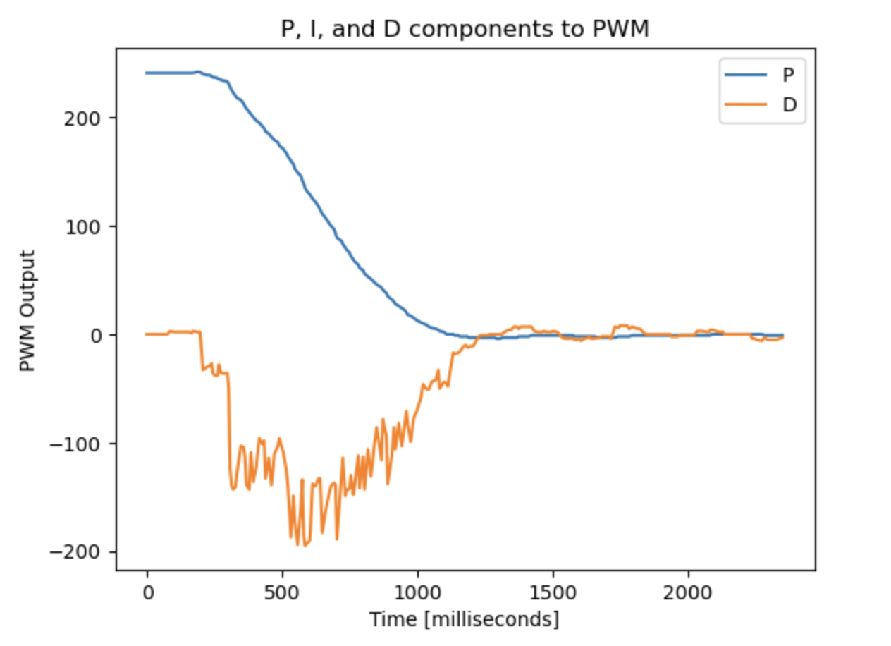
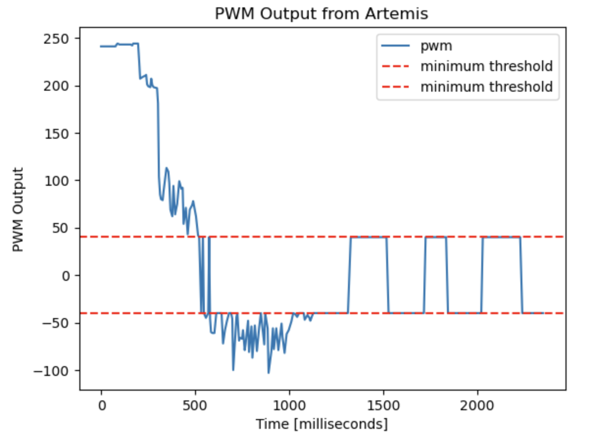
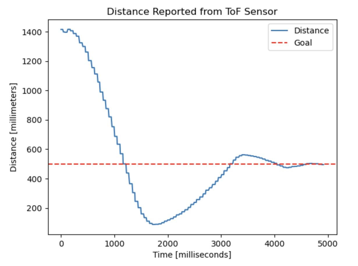
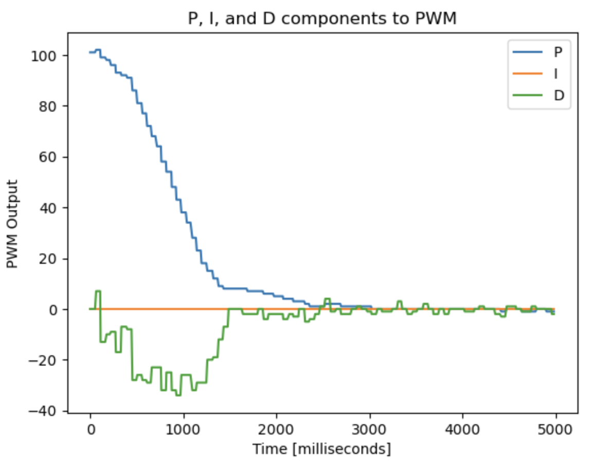
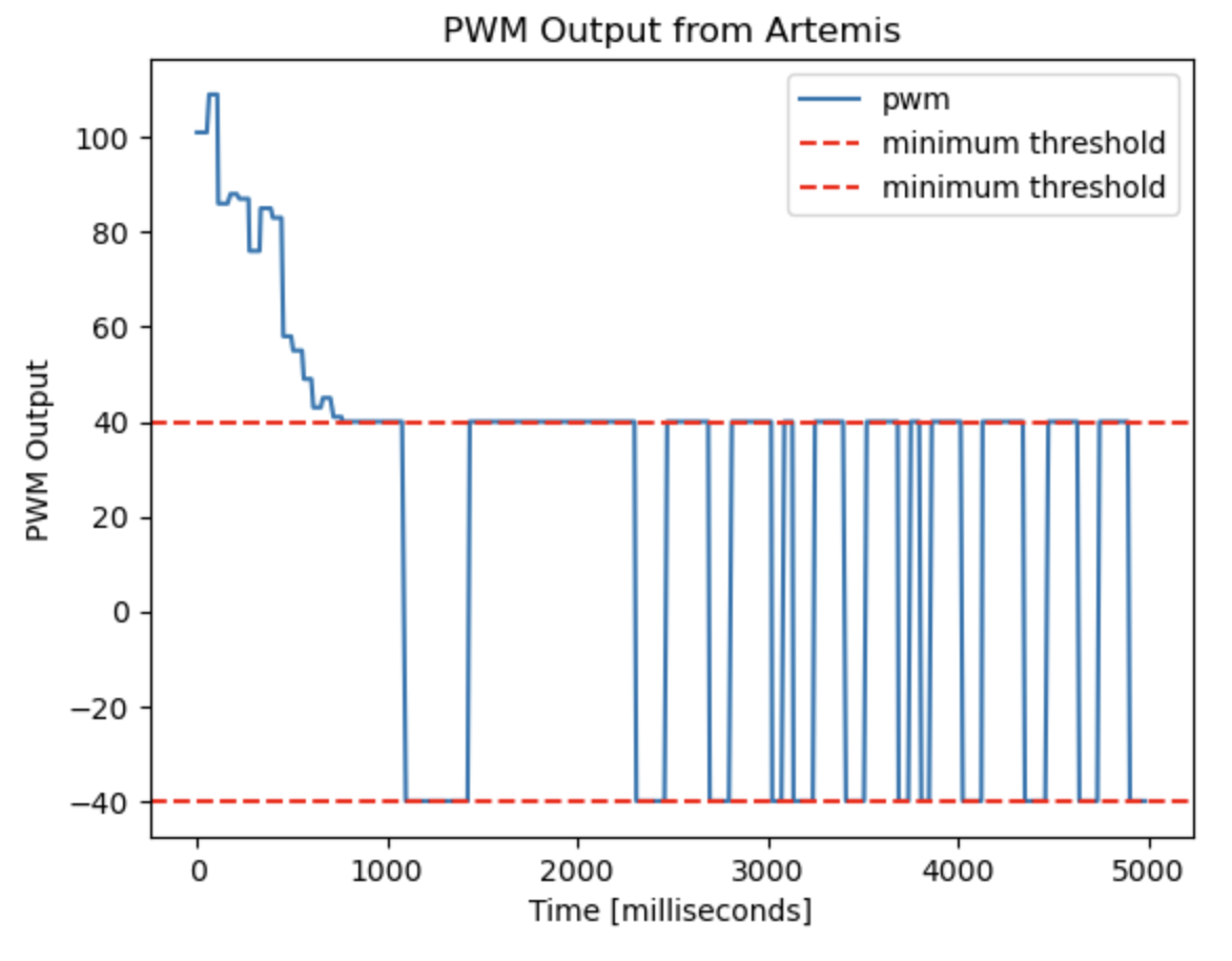
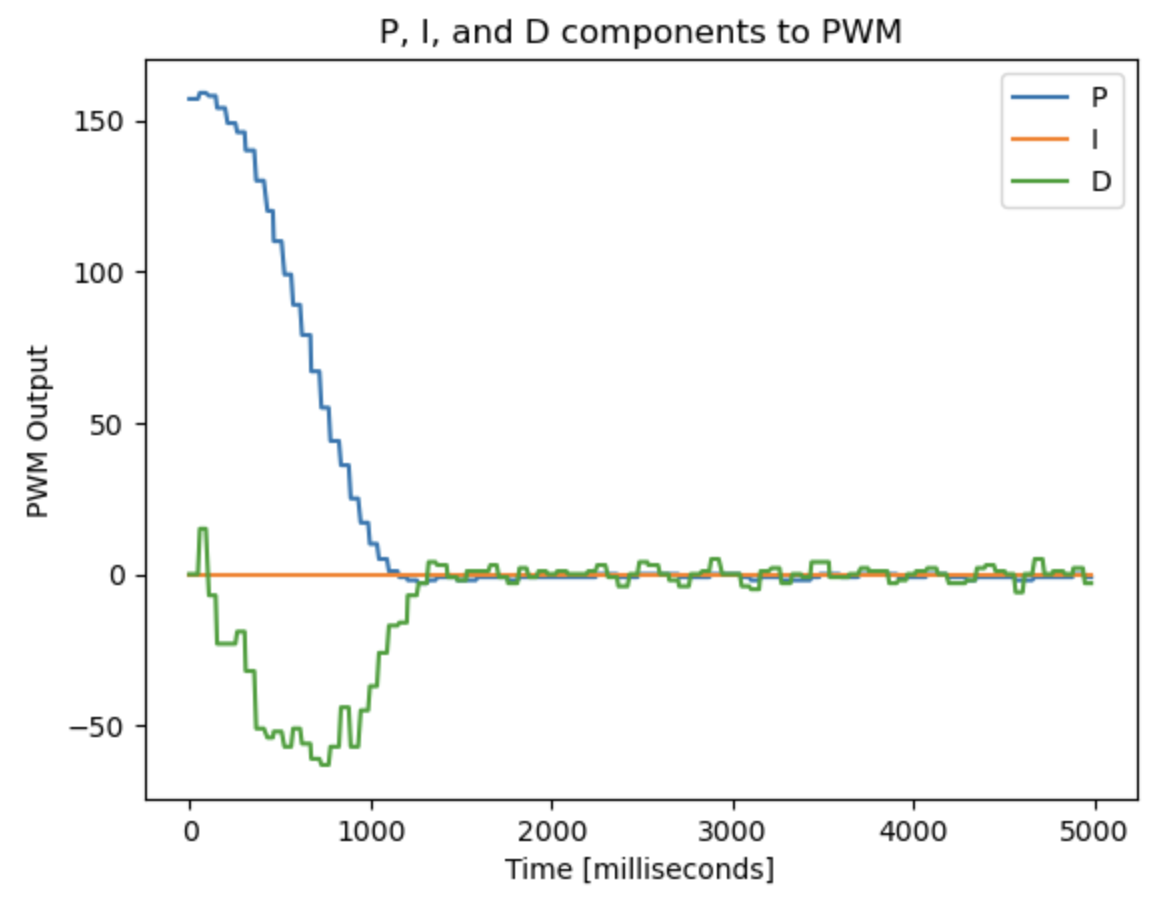
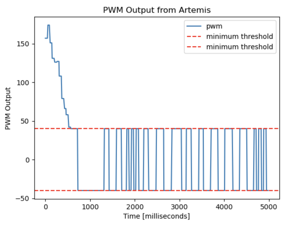
With kp=0.12, and ki=kd=0.0, the car moved slowly and would overshoot the setpoint. This caused oscillatory behavior, which can be seen in the data below. Any PWM output generated that had a magnitude less than 40 was moved to either -40 or 40, depending on the sign of the original output, in order to avoid the deadband region.
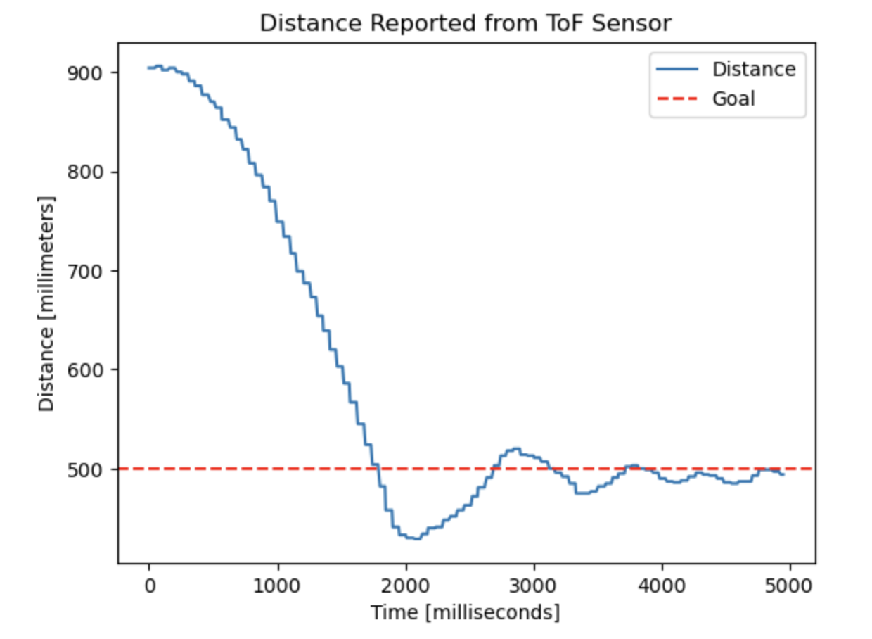
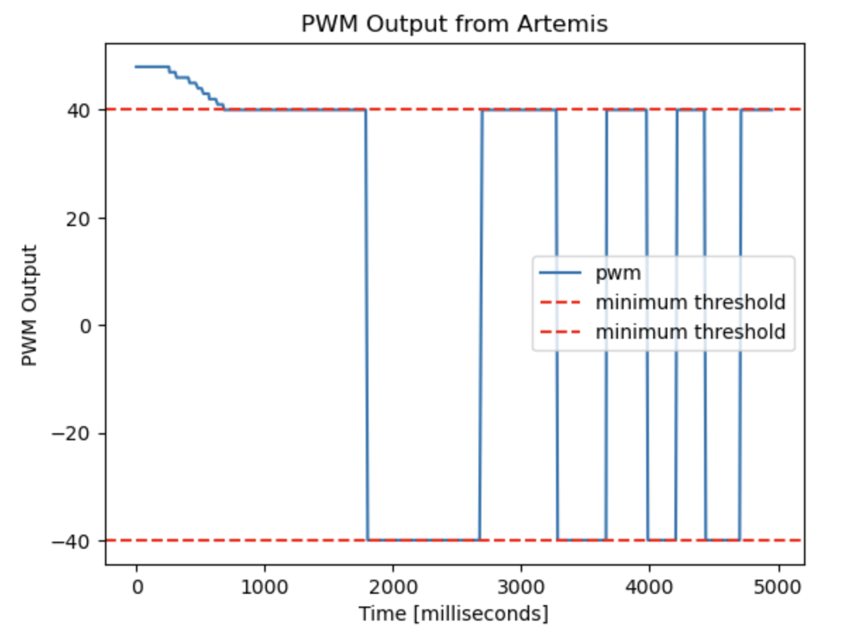
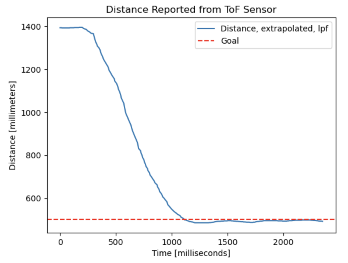
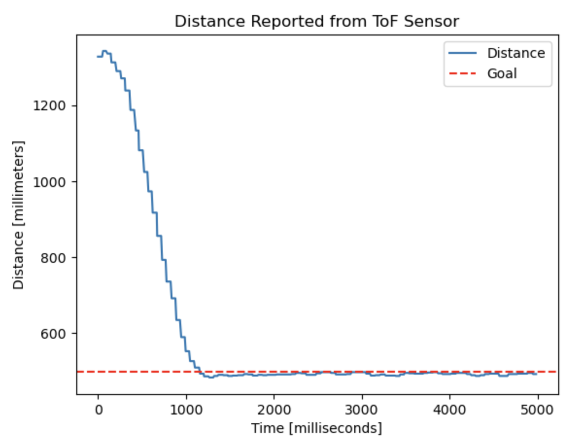
When the initial error was larger, there was more overshoot. Here, the robot starts at about 1390 mm from the wall and is attempting to get to 500mm:
Proportional and Derivative Control
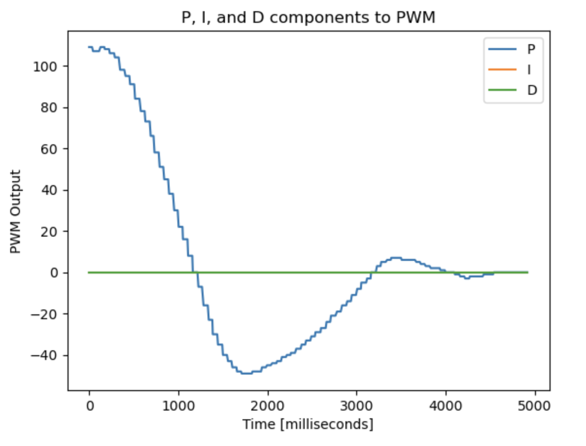
In order to remove oscillatory behavior, I added a non-zero kd term. The derivative term resists changes in the system, acting as a stabilizing component in the control loop. My initial combination of kp and kd values caused the car to reach the desired distance much quicker and with less oscillation.
Hoping to achieve an even smaller settling time, I began to play around with the values of kp and kd. Eventually, I decided that kp = 0.19 and kd = 0.007 produced a quick response from the car with minimal oscillations.
Integral Control
While tuning kp and kd, I noticed that the car never had steady state error between its desired state and its current state. Therefore, I decided that it wasn’t necessary to implement an integral component in the PID controller.
Sampling Time Discussion
The car is very fast, so it’s best to run the controller even faster. If the controller only ran when sensor data was available, it would be significantly bottlenecked by the sampling frequency of the ToF. In order to determine how quick this is, I implemented the following loop on the Artemis:
void
loop()
{
    distanceSensor0.startRanging();
    counter = 0;
    currentMillis = millis();
    loop_stop_time = currentMillis + 60*1000;

    while(millis() <= loop_stop_time){

        if (distanceSensor0.checkForDataReady()) {
            distance = distanceSensor0.getDistance();
            distanceSensor0.clearInterrupt();
            distanceSensor0.stopRanging();
            distanceSensor0.startRanging();
            counter = counter + 1;
        }
    }
    Serial.print((loop_stop_time - currentMillis)/1000);
    Serial.print(" seconds, ");
    Serial.print(counter);
    Serial.print(" reads, ");
    Serial.print(counter/((loop_stop_time - currentMillis)/1000));
    Serial.println(" frequency");
}
On average, the sampling rate of the ToF sensor was about 33 Hz. The maximum sampling frequency of the ToF is 50 Hz when in the short distance sensing mode, validating that my system is within the expected range of operation. Even if the ToF sampled at 50 Hz, this frequency is too slow to run the control loop at.
Decoupling Sensor and Control Frequency
A basic way to decouple the sensor sampling and control frequency is to do your control logic on the most recent sensor data reading until new data is available. However, this assumes that the distance from the car to the obstacle in front of it is constant between sensor measurements, which is not physically realistic if the car is moving.
Alternatively, we can linearly extrapolate the two most recent sensor readings whenever the ToF sensor is not able to provide an updated sensor reading. This assumes that modeling the velocity as constant between sensor readings, which is more realistic than the previously described method.
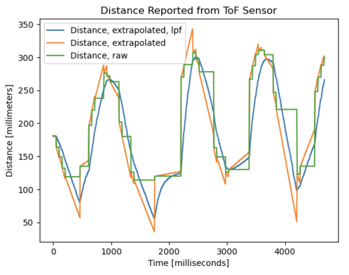
Through this extrapolation, I was able to generate distance data whenever necessary. While this new data often closely followed the true distance, it became very inaccurate when the robot car switched which direction it was moving in. This can be seen in the graph below:
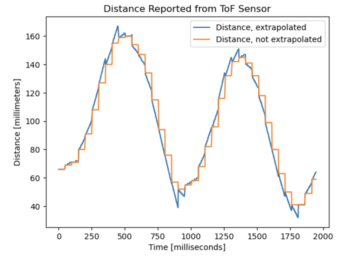
These jagged changes caused incredible noise in the derivative term, so I passed the extrapolated data into a low-pass filter. To prevent too much delay from filtering, I implemented a weaker low-pass filter that smoothed most of the data but didn’t avoid all of the noise. This can be seen in some of the peaks in the data below:
By extrapolating the distance data, I was able to decouple the sensor sampling frequency with that of the controller, which ran at about 110 Hz.
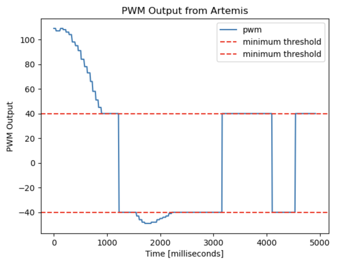
System Performance with Extrapolated Data
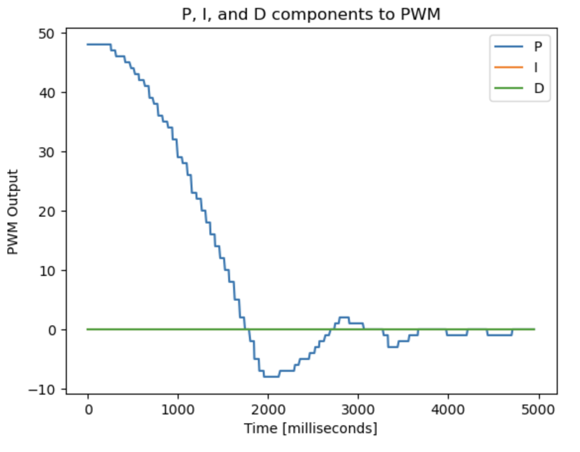
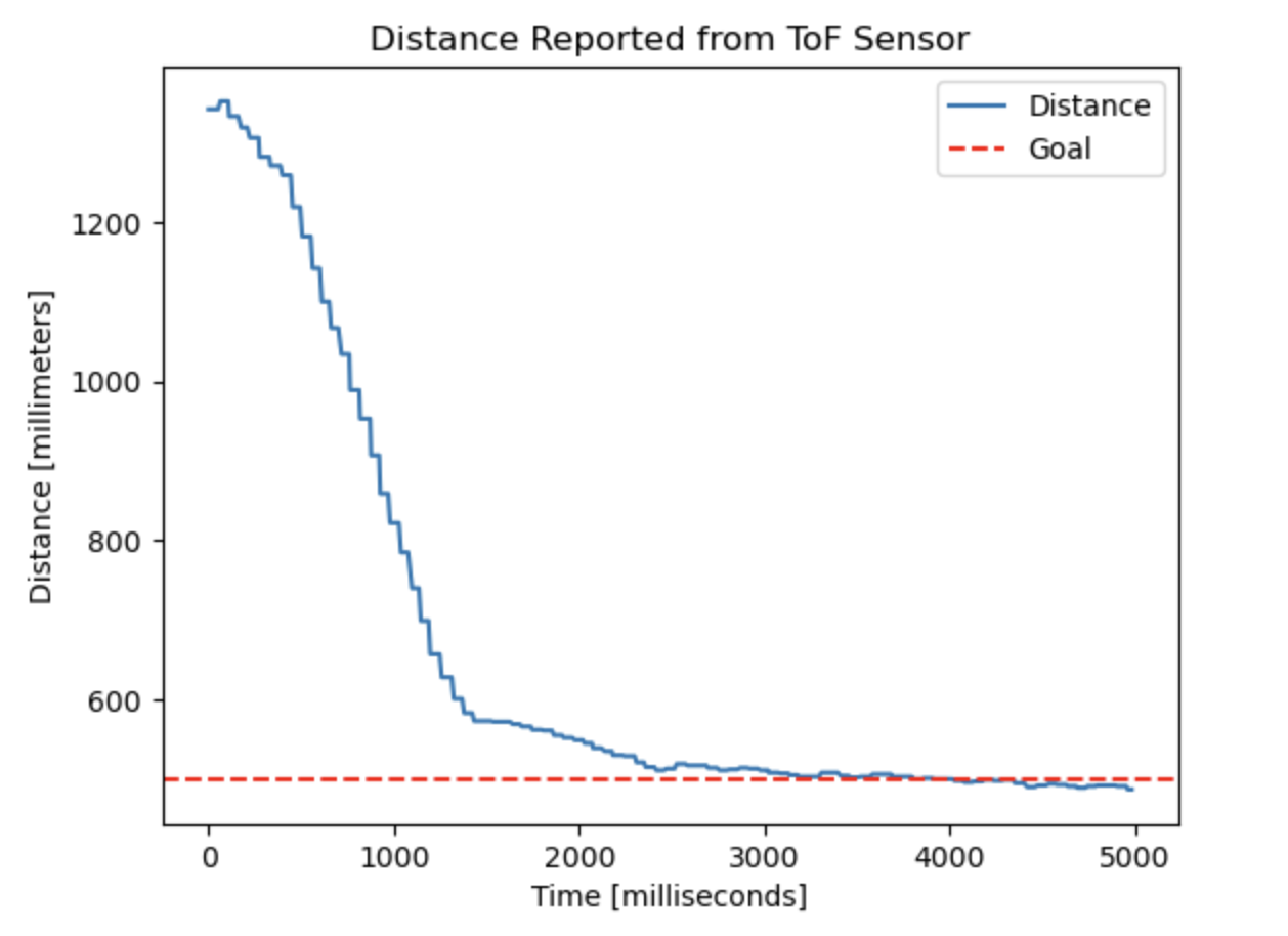
After implementing this extrapolation, I found that the system was not as quick as it had been. In order to speed it up, I experimented with new values for kp and kd, eventually choosing kp = 0.27 and kd = 0.11.
The performance of the robot with the extrapolated data is comparable to without it. This can be seen in the video and graphs below: