Lab 3: Time of Flight Sensors
Prelab
I2C Communication Overview
There are different types of communication protocols between sensors and microcontrollers like the Artemis Nano, but a major one is the I2C protocol. In I2C, all sensing devices share a serial clock line, a serial data line, power, and ground. All of the connected devices send and receive data from the controller along the shared data line, which greatly decreases the number of physical connections the sensors need to make with the microcontroller, as opposed to a SPI communication protocol where every sensor needs its own communication lines.
Due to the fact that many devices can share one I2C bus, each of these devices must be uniquely addressable by the microcontroller. This allows the controller to indicate which device it wants to write/read data to/from, and then that particular device can acknowledge that it is ready to receive/send data. Then communication between the controller and device can take place. However, it is common to have multiple sensors with the same address. For example, in this lab, the IMU has a unique I2C address of 0x69, but both Time of Flight (ToF) sensors have the same default address.
Interestingly, while the documentation for the ToF sensors says that they have an I2C address of 0x52/0x53, their actual default address is 0x29. This will be explained in the I2C Addressing section below. Both ToF sensors sharing the same address presents an issue when wanting to create a system that uses them simultaneaously, and solutions to this problem are discussed below.
Using Two Time of Flight Sensors
The ToF sensors communicate with the Artemis board through an I2C communication protocol. As mentioned above, in order for the microcontroller to communicate with all powered, connected devices, each sensor must have a unique I2C address. This becomes an issue when using two ToF sensors that have the same default address, and there are two ways of overcoming this communication obstacle.
The first method to provide stable communication to both of the ToF sensors doesn’t require the devices to have unique addresses. Devices only need to have unique addresses on an I2C bus if the controller is trying to communicate with said device, and this communication can only take place if that sensor is powered. Therefore, if the controller powers down one of the sensors with duplicate addresses when trying to read from the other sensor, there will be no addressing issues. After collecting the data of interest, the controller can turn the powered off device back on. Both devices can stay on until the controller wants to communicate with one of them again, at which time it would turn the other device off.
The second method requires you to turn a sensor off only once. During the setup of the program, if one of the sensors are turned off and can’t communicate with the controller, then the program can actually change the address of the other identical device. By changing the address of one of the ToF sensors, there will no longer be a communication issue, and both devices can continuously be powered through the duration of the program.
I chose to implement the second solution, as it requires only a little bit of computation at the setup of the program to fix the communication issue, as opposed to constantly turning devices off and on at a high pace.
In order to turn the second ToF sensor off while changing the address of the first, I set the XSHUT pin on the second ToF sensor low. This pin places the sensor into hardware-shutdown, making it invisible to the controller, and now there is only one device with the original duplicated address alive on the I2C bus. This allows me to set a new address for the first sensor, different from its original address and that of the IMU. This is shown in the code snippet below:
digitalWrite(SHUTDOWN_PIN, LOW); // turns ToF sensor 1 off
int add;
add = distanceSensor0.getI2CAddress(); // gets the original I2C address
Serial.print("The old address of sensor 0 is: ");
Serial.println(add);
distanceSensor0.setI2CAddress(0x40); // sets a new I2C address
add = distanceSensor0.getI2CAddress();
Serial.print("The new address of sensor 0 is: ");
Serial.println(add);
digitalWrite(SHUTDOWN_PIN, HIGH); // turns ToF sensor 1 back on
Sensor Placement
In our lab kit, we were given four QWIIC connect wires, two of which were almost twice the length of the other two. This prompted me to think about how the sensors should be laid out on the robot before soldering two of them to the ToF sensors, which do not have QWIIC connect ports. With an understanding that the robot car has to avoid obstacles that are approaching it from the front, and at some point will have to maintain a specified distance from a wall to its side while driving forward, I thought that the optimal placements of the ToF sensors would be on the front and side.
I thought that the accelerometer should be as close to the center of the robot as possible, since the car implements differential drive, and this would be the center of the car’s rotation. The picture below shows a sensor layout next to the robot car to illustrate their relative sizes. The two green sensors are the ToF sensors. I decided to connect one of the ToF sensors to a longer QWIIC connector and the other to a short one so that the ToF sensor in the front of the car has a farther reach. The ToF sensor on the side of the car is closer to the center of the car, where the IMU will also be, so both of those sensors can use the shorter QWIIC connector wires.
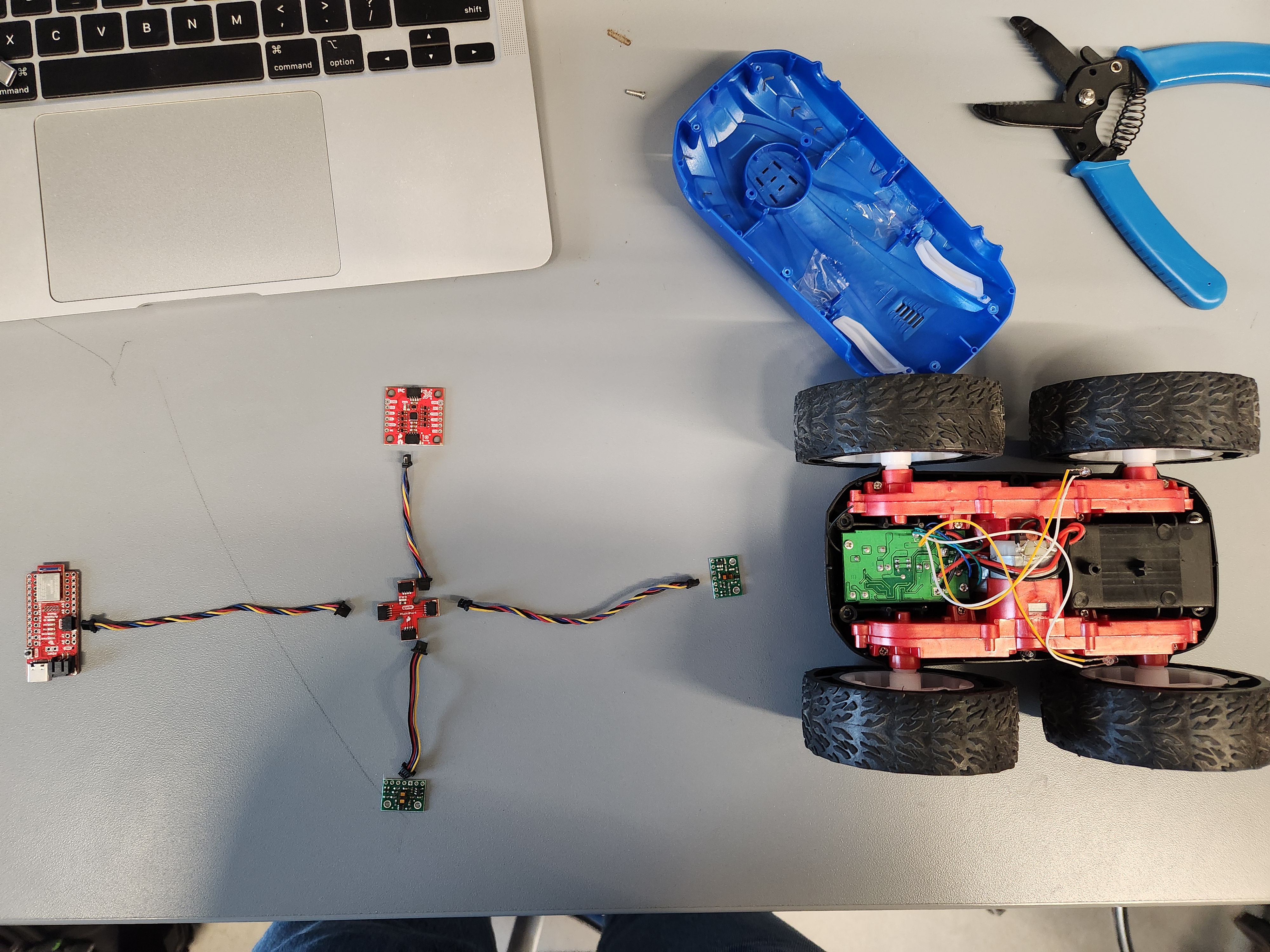
This setup, however, will not allow the robot to detect objects on at least two sides of its chassis. This could make it possible that the robot could turn or back into an object it had not previously detected, so this will have to be kept in mind when developing the control algorithm for this car.
Wiring
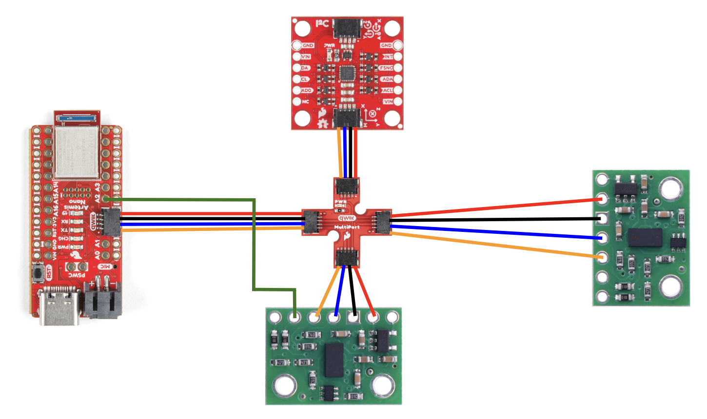
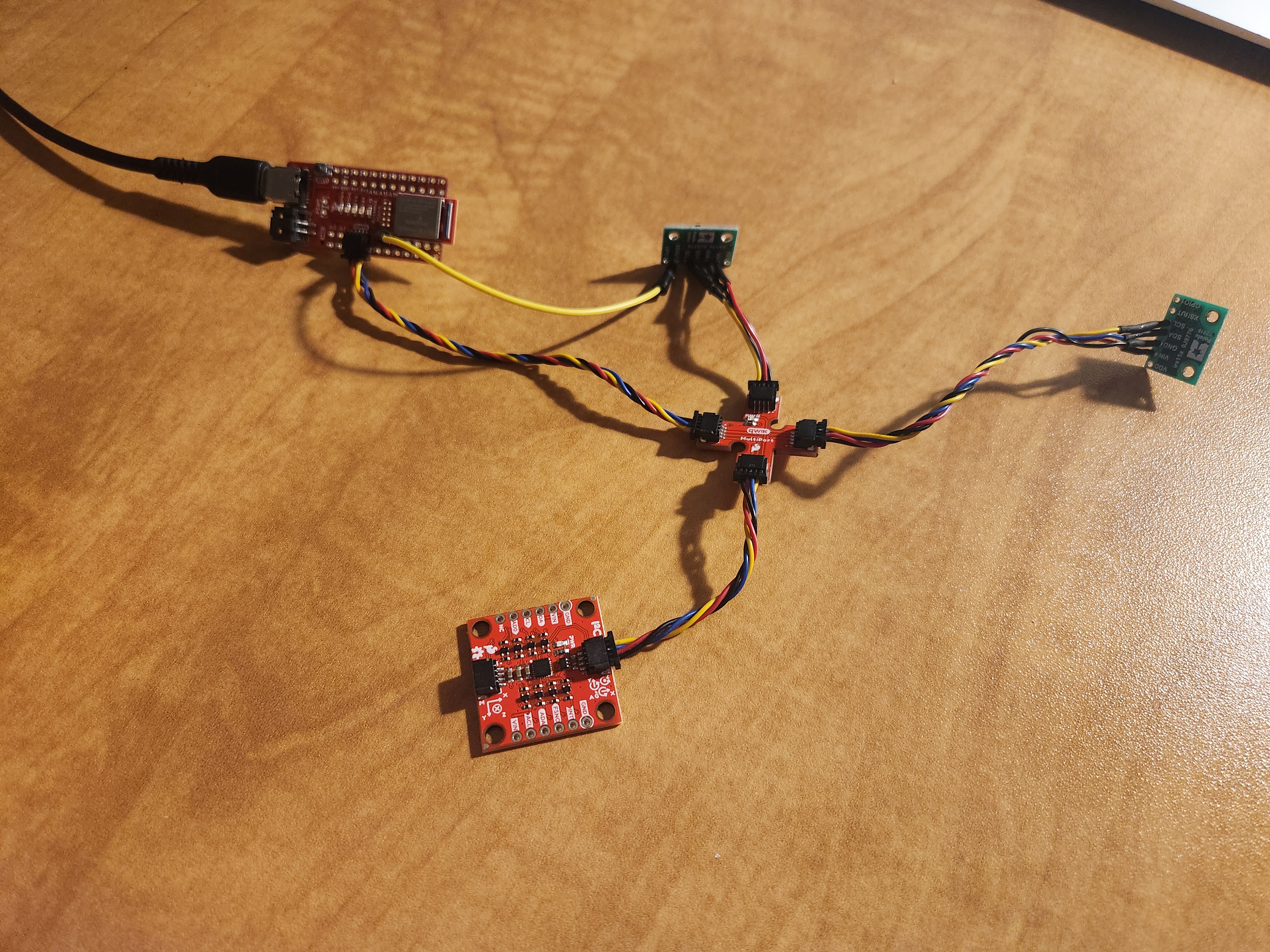
Here is the wiring diagram, as well as the finished wiring connections.
Lab Tasks
I2C Addressing
When the Artemis scans for I2C addresses from devices connected to it, the following output is printed when one IMU and one ToF sensor are present connected to it.
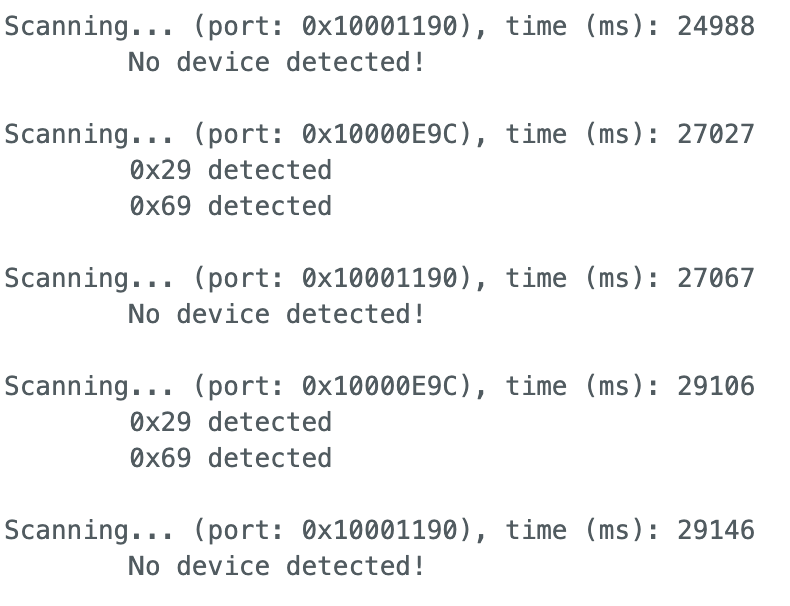
This output shows that on the first I2C bus, there are no I2C devices connected to the board. This makes sense, as we are connecting both the IMU and the ToF sensors to the same port. The output shows that the second I2C bus has two devices on it, with addresses 0x29 and 0x69. The device with address 0x69 is the IMU, which can be determined by looking through the IMU datasheet. But what is the device with address 0x29?
The documentation for the ToF sensor indicates that default I2C address is either 0x52 or 0x53, depending on if the controller is writing or reading from the sensor. However, when scanning for I2C devices connected to the Artemis board, the program reported that the address of the ToF sensor was actually 0x29. These are very different addresses, and they do not look remotely similar in neither hexadecimal nor decimal.
When these addresses are represented in binary, however, they look more similar. In binary, 0x52 becomes 0b1010010, 0x53 becomes 0b1010011, and 0x29 becomes 0b101001. These are very similar, with 0x29 being 0x52/0x53 shifted one bit to the right. While this might initially seem odd, it makes sense when thinking about these numbers as a combination of digital addresses and commands used on the I2C bus. The controller outputs a sequence of binary signals in order to indicate what device that it would like to communicate with on the bus. This code indicates that this address would be 0b101001 for the ToF sensor. But then why would the addresses be reported as 0x52/0x53 in the documentation?
By further looking into the sensor’s documentation, it can be seen that if the least significant bit of the address is low, then the controller is indicating that it wants to write to the sensor. If the least significant bit is high, then the controller wants to read from the sensor. The true address of the ToF sensor is 0x29, and this shouldn’t automatically change depending on if the controller is executing a read or write command. Therefore, it seems that the true address of the sensor was shifted left by one, creating a new least significant bit that did not contain address information, and this could be changed to indicate how the controller wants to interact with the sensor.
ToF Sensing Characteristics
The ToF sensor comes with two available sensing modes: short distance and long distance. The short distance method focuses on accurately measuring distance up to 1.3 meters away from the sensor, and the long distance mode tries to accurately measure up to 4 meters away. Whichever mode the sensors are placed in is completely up to the programmer, creating a need to compare their benefits and costs.
The short distance sensing mode can be more accurate, as it is discretizing a smaller allowable range of data. However, this accuracy is only applicable for distances close to the sensor, meaning that the sensor may miss important data coming from obstacles or objects that are outside of its range of accurate detecting. This can cause systems using the short distance method to not be able to plan much in advance to avoid obstacles, and they will need to be able to adapt to data faster as they will have to get physically closer to objects to accurately detect them.
The long distance sensing mode has a larger range, allowing systems using it to quickly react to onjects that are farther away from it. This could be good for my car robot because it could detect obstacles or walls sooner. However, this increased range corresponds with a less accurate measurement, and any increased error in measurement could have negative effects on the state estimation and controls of the robot. Additionally, ranging over a longer distance means that it would take more time to make measurements, slowing down the sampling rate of the sensor.
Since the goal of this class is to develop a fast robot car, speed and accuracy is paramount. The car has very fast dynamics, being able to change heading, direction, and speed incredibly quickly. Therefore, this system should be quick enough to adapt to rapidly incoming data about its environment, so I will use the short distance measurement mode for the ToF sensors. While this mode is only optimal in a smaller range of distances, it is more accurate and faster than the long distance mode.
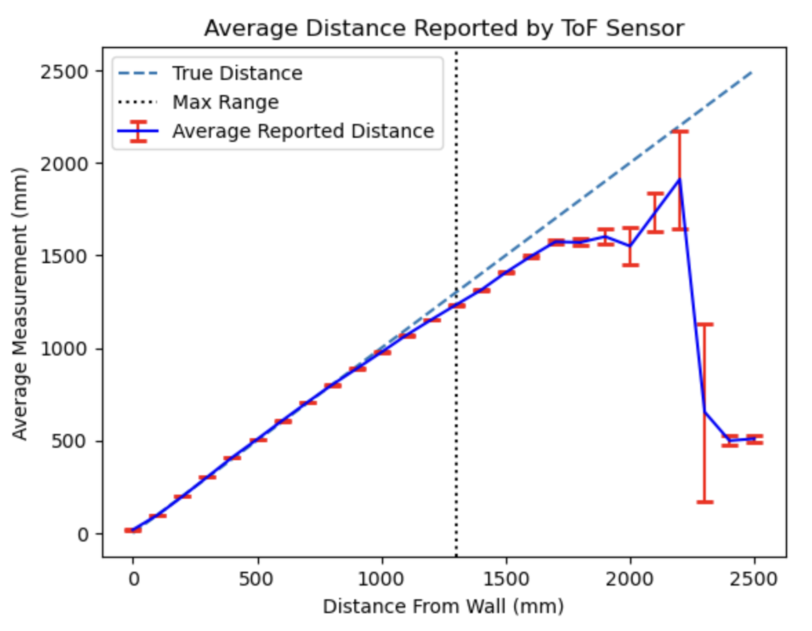
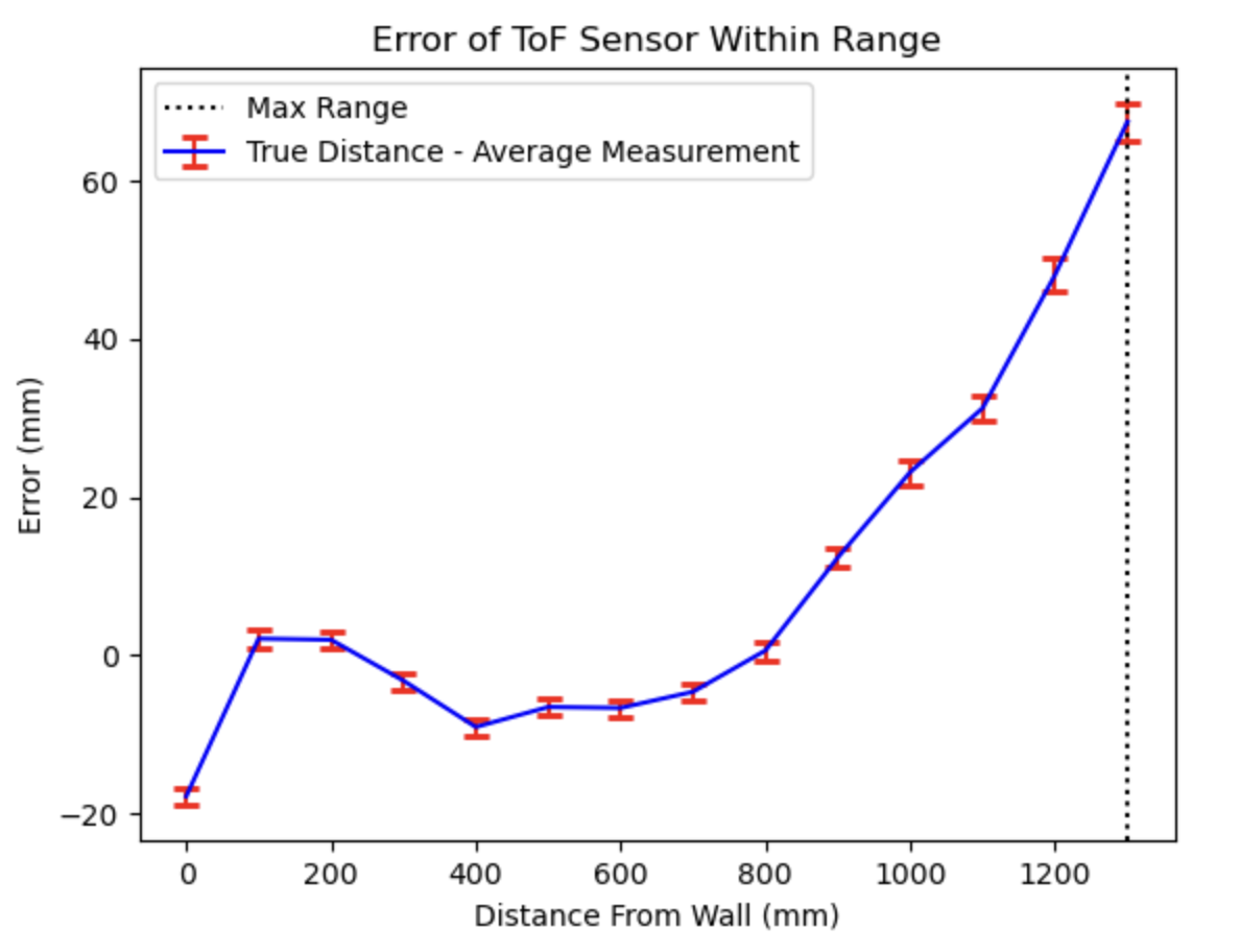
To test the accuracy and range of the ToF sensor, I created an experiment that took many ToF measurements at various distances from a wall and then looked at the results of these measurements. To do this, I taped a single ToF sensor to the front of a box, such that it was perpendicular to the floor and was pointing directly at the wall in front of the box. Using a tape measure, I placed the box with the ToF sensor taped to it at known distances from the wall. Once the box had been placed in position, I took thousands of ToF sensor readings without moving the box. I averaged these values, found their standard deviation, moved the box a little bit further away from the wall, and repeated the whole process for distances from 0 m to 2.5 m away from the wall in 0.1 m intervals.
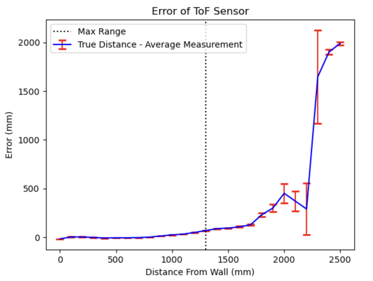
The first two graphs below depict the average measured data from the ToF sensor at various fixed distances from a wall, as well as the error between the true distance from the wall and the measured distance. Notice how the accuracy of the sensor dramatically decreases past the maximum ranging point for the short distance method, which is 1.3 m.
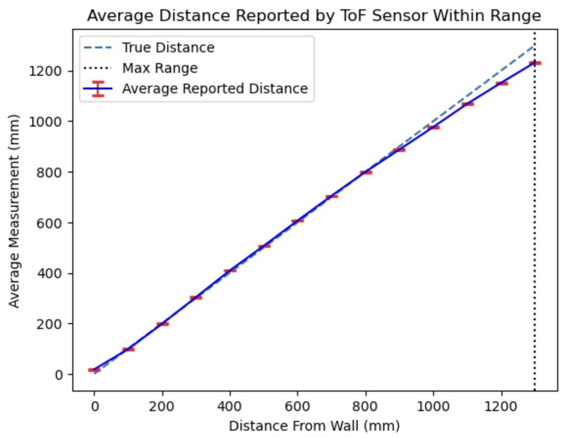
These two graphs show the same data as above, but zoomed in around the operating range of the ToF sensor when in the short distance measuring mode.
ToF Speed Characteristics
In order to determine how fast a microcontroller can collect data from the robot’s environment, it is important to determine how fast the ToF sensors can report new distance measurements. This can be tested by running a continuous loop that prints the time, and prints the distance data whenever it is available from either sensor. For clarity, this is shown below.
if (distanceSensor0.checkForDataReady()) { // Checks if ToF sensor is ready to report data
 distance = distanceSensor0.getDistance(); //Get the result of the measurement from the sensor
 distanceSensor0.clearInterrupt();
 distanceSensor0.stopRanging();
 distanceSensor0.startRanging(); // start sensing again
 Serial.print("0: "); // print data from sensor 0
 Serial.println(distance);
}

if (distanceSensor1.checkForDataReady()) {
 distance = distanceSensor1.getDistance(); //Get the result of the measurement from the sensor
 distanceSensor1.clearInterrupt();
 distanceSensor1.stopRanging();
 distanceSensor1.startRanging(); // start sensing again
 Serial.print("1: ");  // print data from sensor 0
 Serial.println(distance);
}

Serial.println(millis()); // print the time since bootup to measure speed of the loop
The execution of the above program outputs a large amount of data. By analyzing the timing of this data, I found that the loop ran at about 570 Hz, and that the ToF sensors reported values at a rate of about 31 Hz. Clearly, the ToF sensors operate at a much slower frequency than the larger loop logic and are the limiting factors in this system.
Additional testing was done to determine the sampling speed of the ToF sensors when operating within a Bluetooth command in order to determine the timing effects of the stopRanging() method. This method, carried out on the ToF sensors after they make a measurement, stops the sensors from taking new measurements. After it is called, the sensor stops sensing its environment until the startRanging() method is called. I found that using the stopRanging() function sped up the sensor’s sampling speed, as shown in the results below. I will therefore continue to use the stopRanging() method.
| Sample Rate with .stopRanging() | Sample Rate without .stopRanging() |
|---|---|
| 50.733 ms | 99.88 ms |
Sensors in Parallel
With both of the ToF sensors and the IMU working in parallel, the limiting factor is the rate at which the ToF sensors report new data, as discussed above. Therefore, if the goal is to run the data acquisition loop as fast as possible, then it would be best to not wait for the ToF sensors to be ready to report new data. The question becomes what to do with the data arrays corresponding with the ToF sensors when they are not providing any new data, but the IMU is ready to update.
I found that when a ToF sensor isn’t ready to report new data, but the data acquisition loop is still requesting new data, it is best to simply set the new distance data equal to the previous distance value. While this may not accurately represent the true distances, it is a better approximation given the recent history of the system than what may happen if the contents of the distance arrays are not updated at the same time as the IMU and timing arrays are. For example, if you don’t update these at the same rate, whatever old data may be stored in the ToF sensing arrays could be reported as true data for the current set of measurements. This can cause confusion for the user and controller as the data might become very discontinuous, so it is best to avoid these odd jumps in data by keeping the distance data more stable.
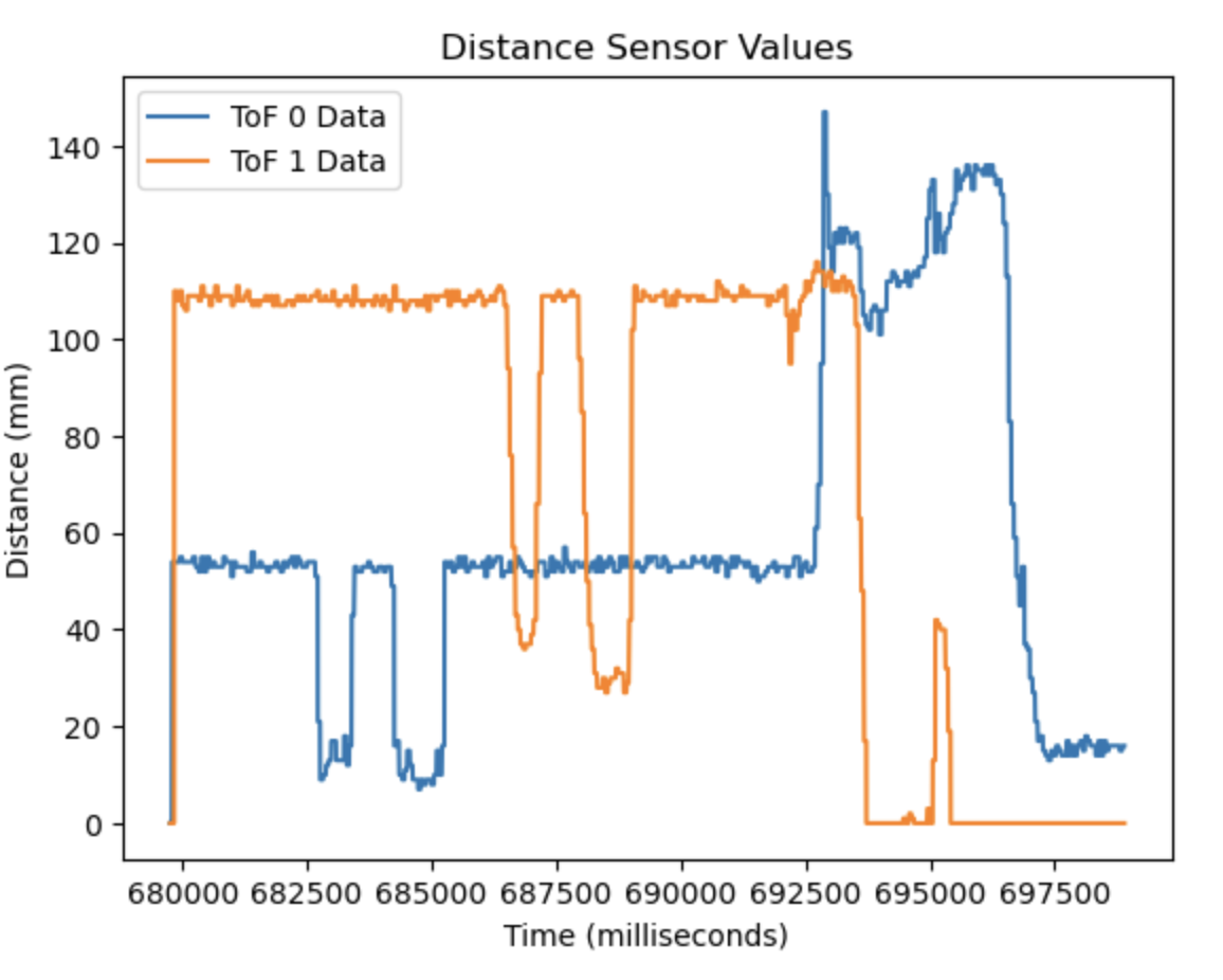
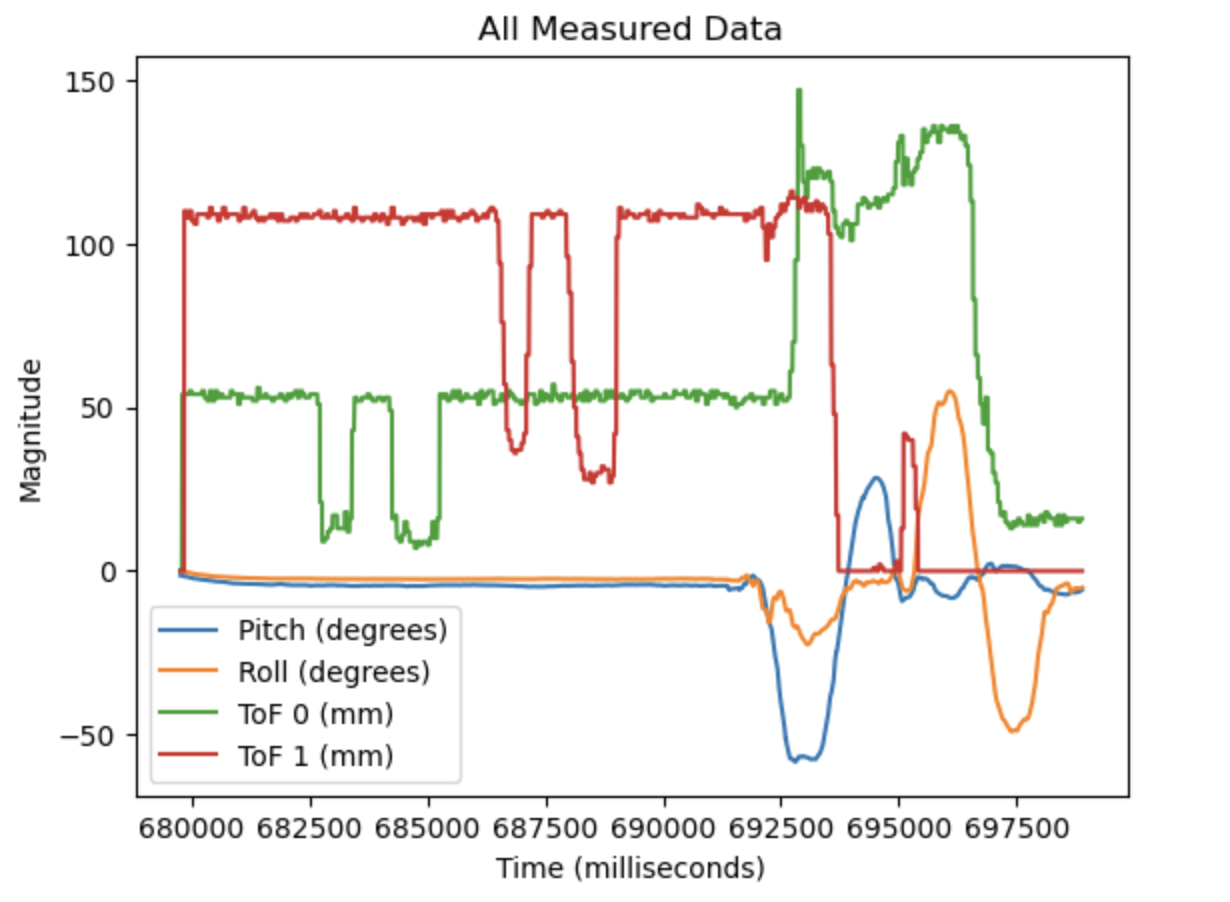
In the video below, you can see me command the Artemis to begin collecting data from the IMU and both ToF sensors through a Bluetooth connection. After starting the data acquisition, I change the data each sensor will report by manipulating them. This can be seen by how I move my hand in front of the ToF sensors to change the distances they read, as well as rotating the IMU to change the calculated pitch and roll.
The results of the above video are included in the plots below. As it can be seen, all of the data is collected on the same timescale, and the disturbances that I made to any of the sensors are represented in appropriate changes of data reported. When moving the IMU, I accidently pulled on both of the ToF sensors, changing their orientation and therefore changing the data that they reported. That is why the distance data becomes noisier when the pitch and roll changes.
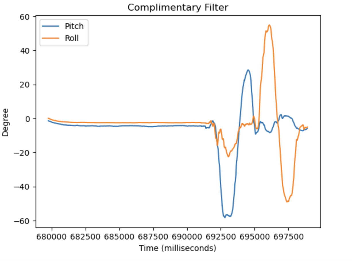
Here is a graph of just the pitch and roll data:
Here is a graph of just the distances measured by the ToF sensors: