Lab 2: Inertial Measurement Unit
Set up the IMU
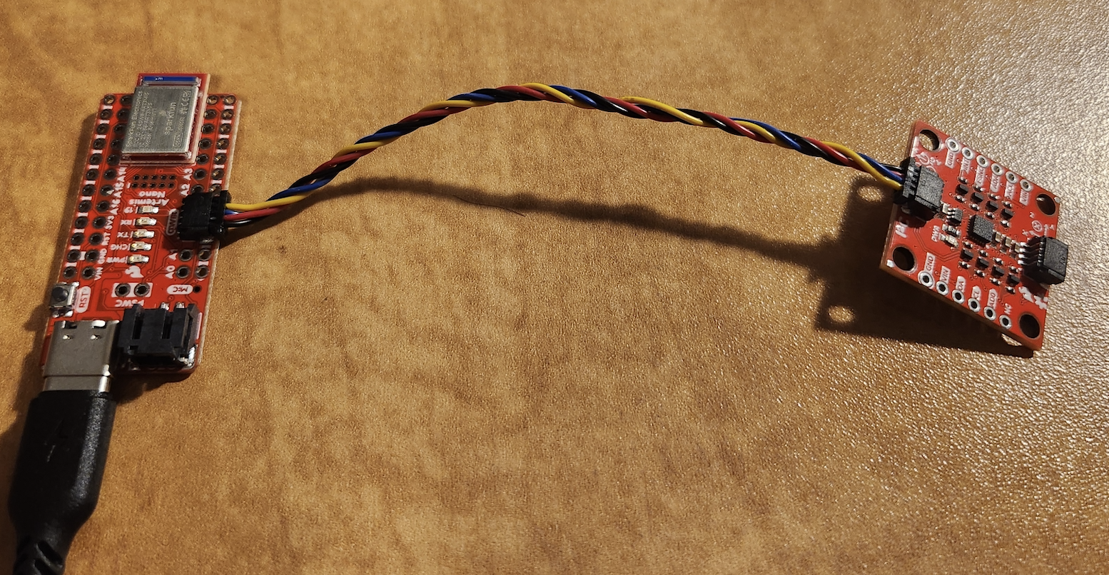
IMU Connections
The IMU connects to the Artemis Nano through a quick connect wire.
IMU Example Code
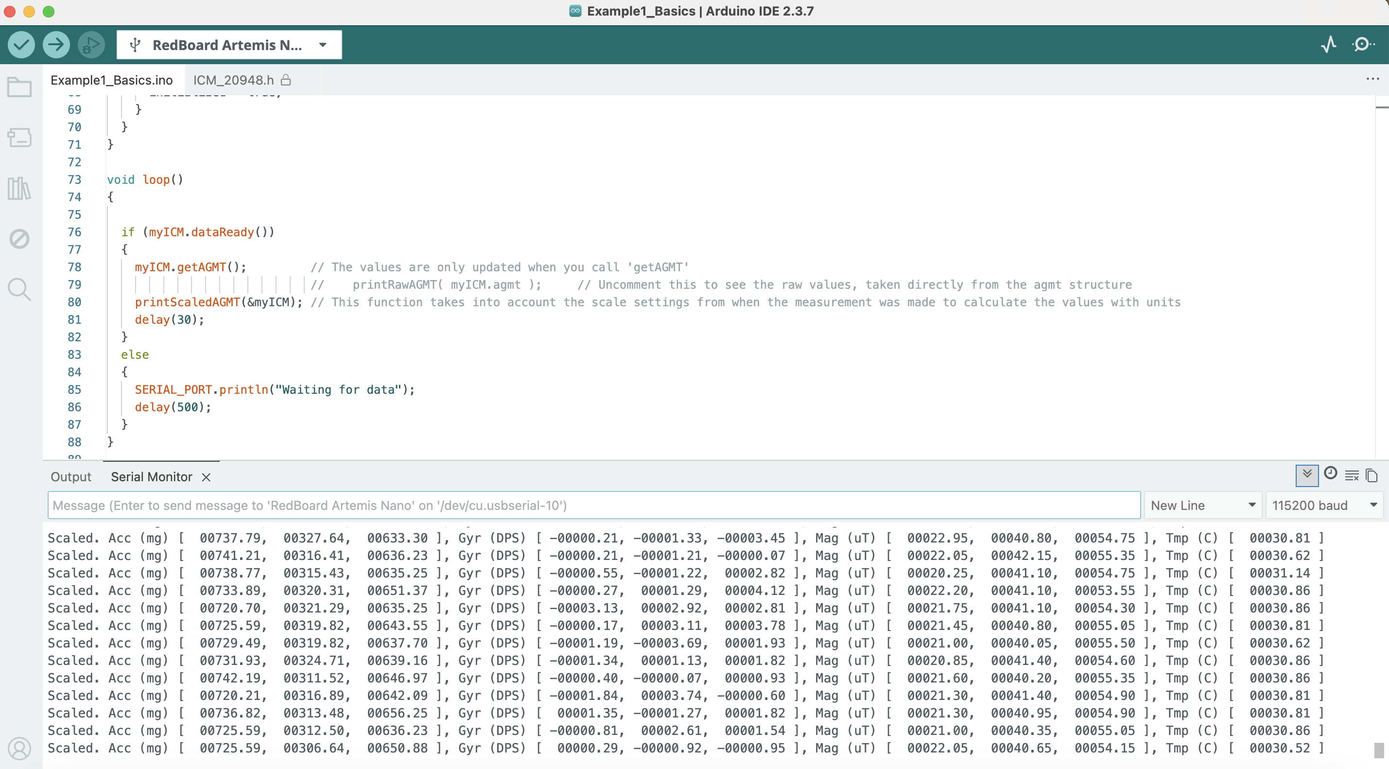
In the ICM 20948 example code, the IMU’s raw values are scaled so that it has proper units with which calculations can be done on. This scaling is necessary because the IMU outputs integer values representing the acceleration, angular velocity, and magnetic field magnitude for all of x, y, and z axes, and without knowing how these seemingly random raw integer values scale to values with units the data is useless.
AD0_VAL Discussion
The value of AD0_VAL is what determines the final address of the IMU. By setting this value either high or low, you can change the address of this device. This is important to know about because this IMU is an I2C device, and every device on the same I2C bus must have a unique address associated with it. This means that you can have two different ICM 20948’s on the same I2C bus because each one can be configured to have different addresses if the AD0_VAL is different for each device. By default, the AD0_VAL should be 1.
Accelerometer and Gyroscope Data Discussion
While running the example code, I noticed that the accelerometer and gyroscope data behaves differently.
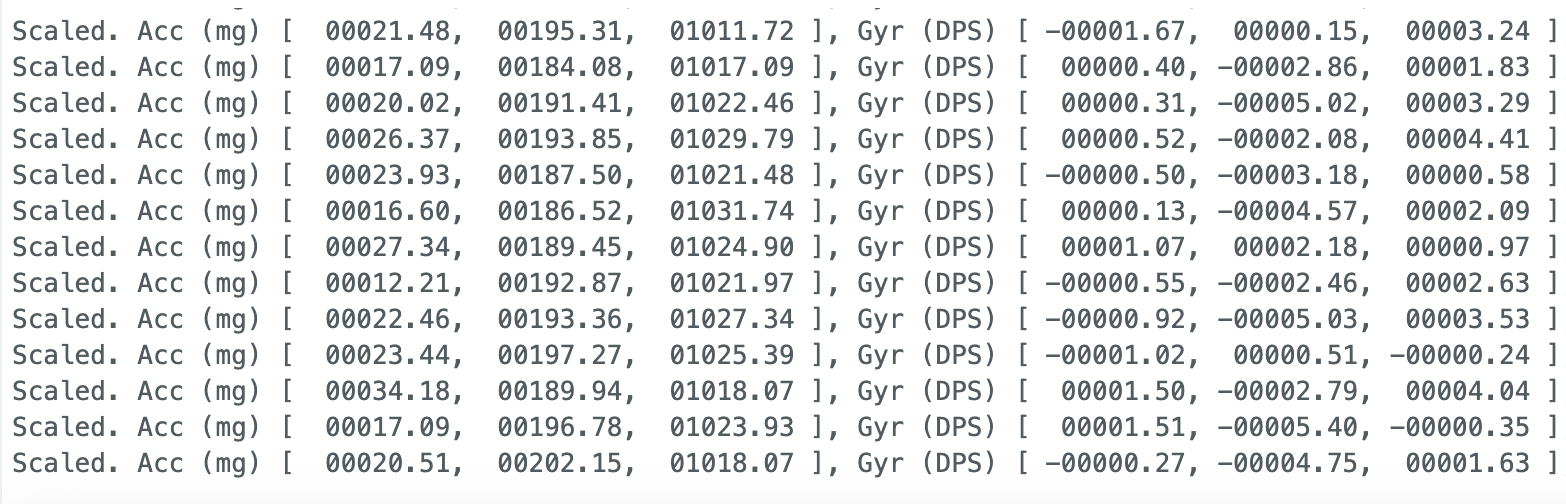
The accelerometer data takes on large values, comfortably ranging from 1000 mg to -1000 mg when not moving and facing upwards or downwards, respectively. When the device stays still, the accelerometer data seems to be a little bit noisy, but the noise is concentrated about some mean value.
On the other hand, the gyroscope only reads large values when the device is rotating about one of its axes. Otherwise, the values are practically zero. This makes sense because the gyroscope measures the change in degree per second, so if the device isn’t rotating then it wouldn’t have an angular velocity.
Here is an image when the IMU is facing upwards.
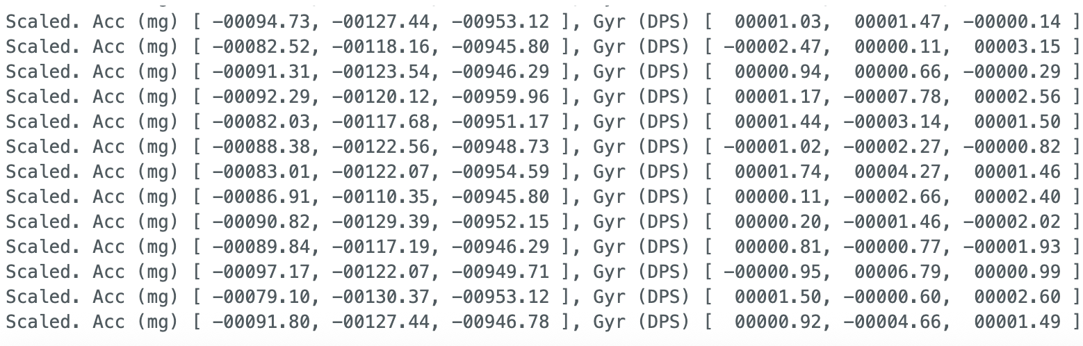
Here is an image when the IMU is facing downwards. Note the change of sign on the z-acceleration component.
Accelerometer
Accelerometer Accuracy
When the accelerometer returns measurements, the precision of the measurements depends on the full-scale range of the IMU, which is programmable. In my program, the full-scale range is such that the accelerometer reports acceleration values between ±2g. This means that a value of 1g is reported as the integer value 16,384.
When the is IMU flat on the table, one would expect the z-acceleration to be +16,384 when facing up, and -16,384 when facing down. My IMU reported about 17,114 when facing upwards and -15,782 when facing down. Assuming that any offset from the expected output is linear, I can determine how far away the data is from the expected values in the down and up position. By averaging these differences and adding this averaged offset to all of the acceleration data, I can make is comparable with what is expected. Therefore, I will subtract about 660 to all acceleration data collected moving forward, a correction of about 0.04g.
Roll and Pitch as Determined by the Accelerometer
In order to calculate the pitch and roll of the IMU, two very simple equations are needed. By using geometry and trigonometry on a simple model of the IMU, it can be determined that the equation to determine the pitch of the IMU is: atan2(x-acceleration, z-acceleration), and the equation for roll is atan2(y-acceleration, z-acceleration).
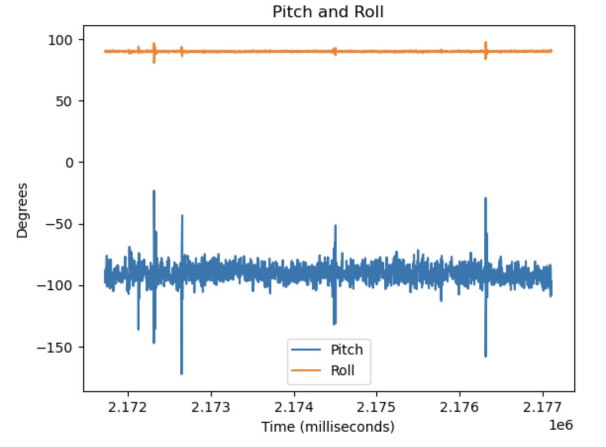
As it can be seen, these two equations are both dependent on the z-acceleration, which couples them and can lead to undesirable effects when the z component approaches 0. This causes either the pitch or roll to diverege when the othe one approaches ±90 degrees. These singularities are due to the mathematical equations of the pitch and roll and are not related to the sensor itself. See below for more examples of this.
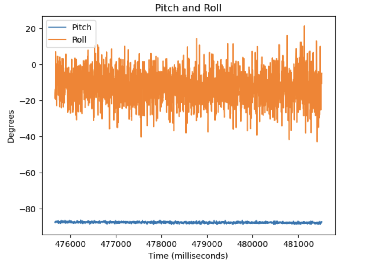
Value of Pitch and Roll when Pitch is positioned at -90 Degrees
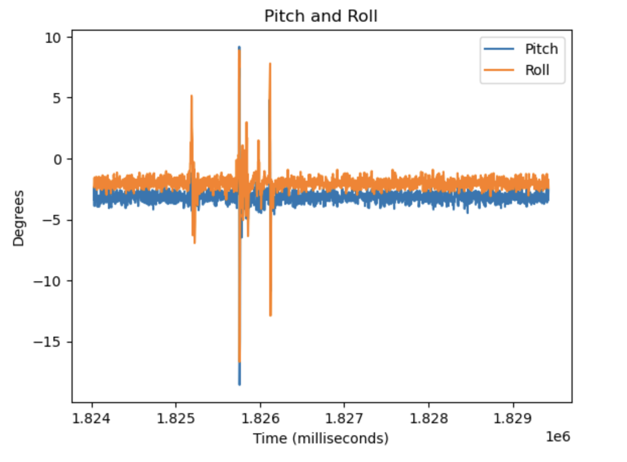
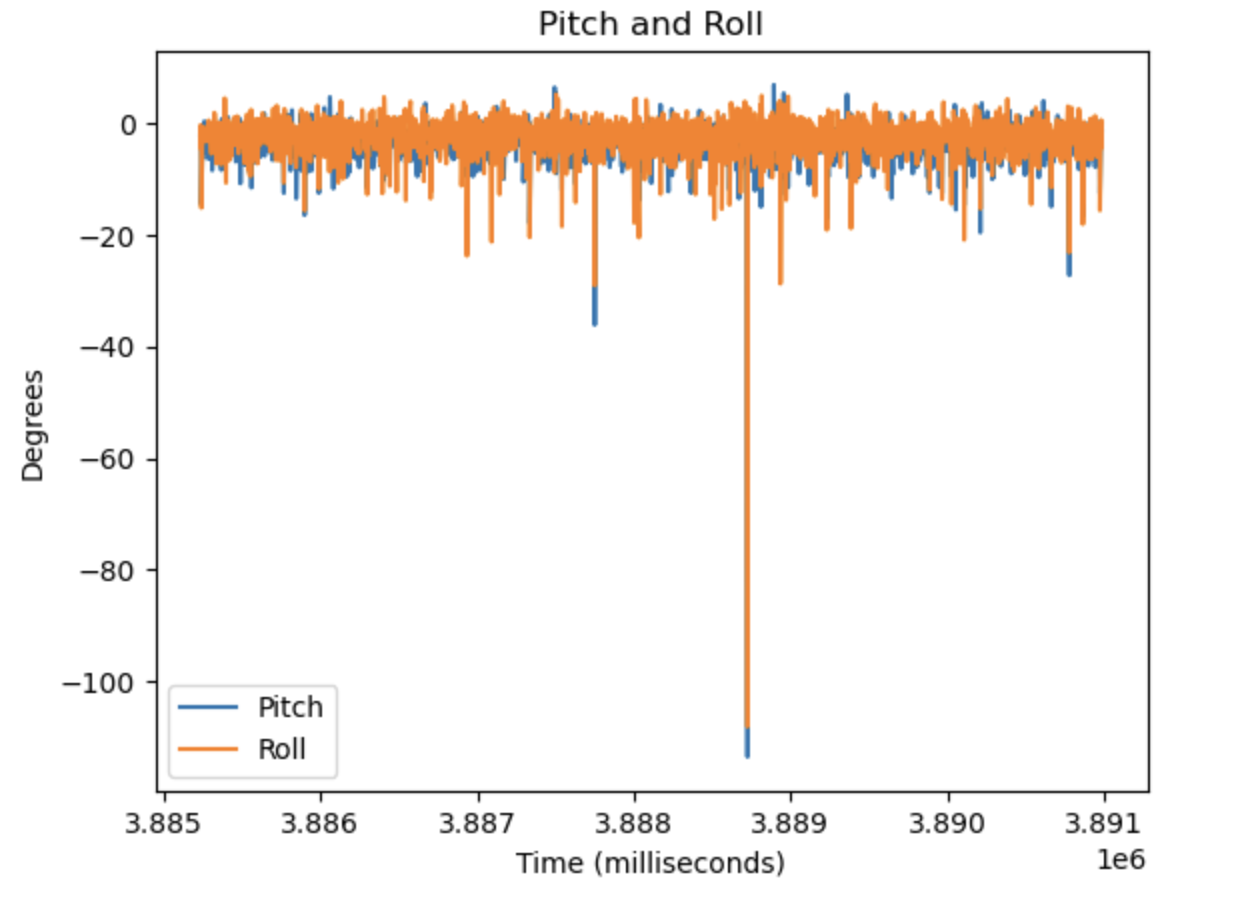
Value of Pitch and Roll when Pitch is positioned at 0 Degrees
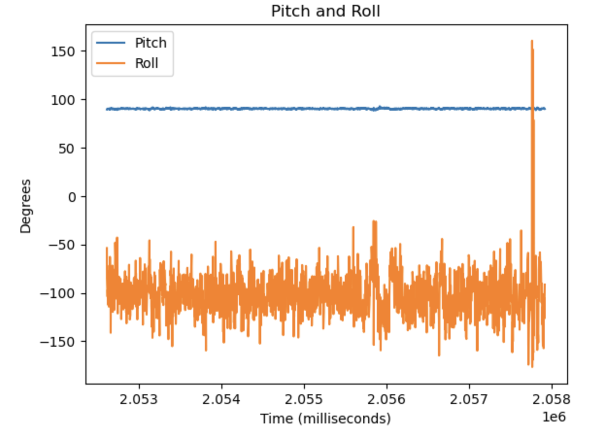
Value of Pitch and Roll when Pitch is positioned at 90 Degrees
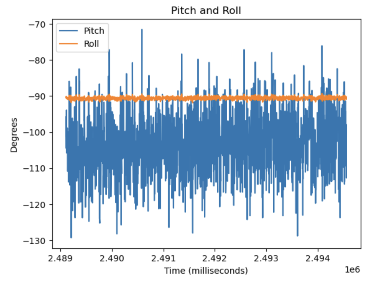
Value of Pitch and Roll when Roll is positioned at -90 Degrees
Value of Pitch and Roll when Roll is positioned at 0 Degrees
Value of Pitch and Roll when Roll is positioned at 90 Degrees
Frequency Analysis
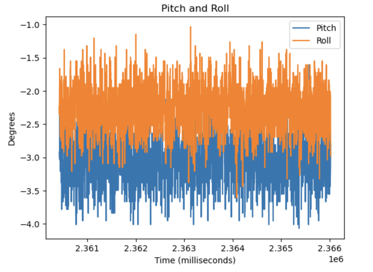
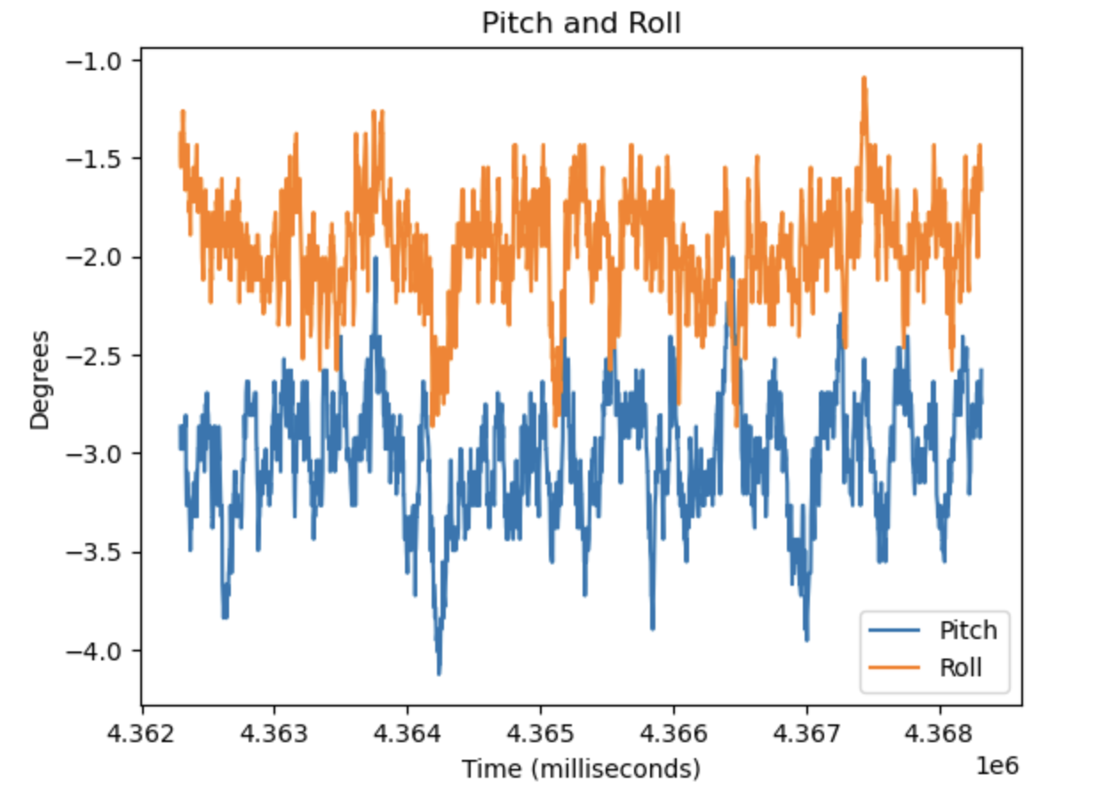
It is very noticeable in the previous graphs that the pitch and roll data are extremely noisy, which is due to the noisy accelerometer data. The image below shows the pitch and roll values when the IMU is flat and motionless on a table.
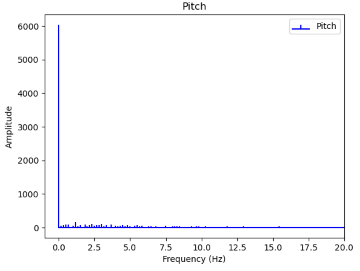
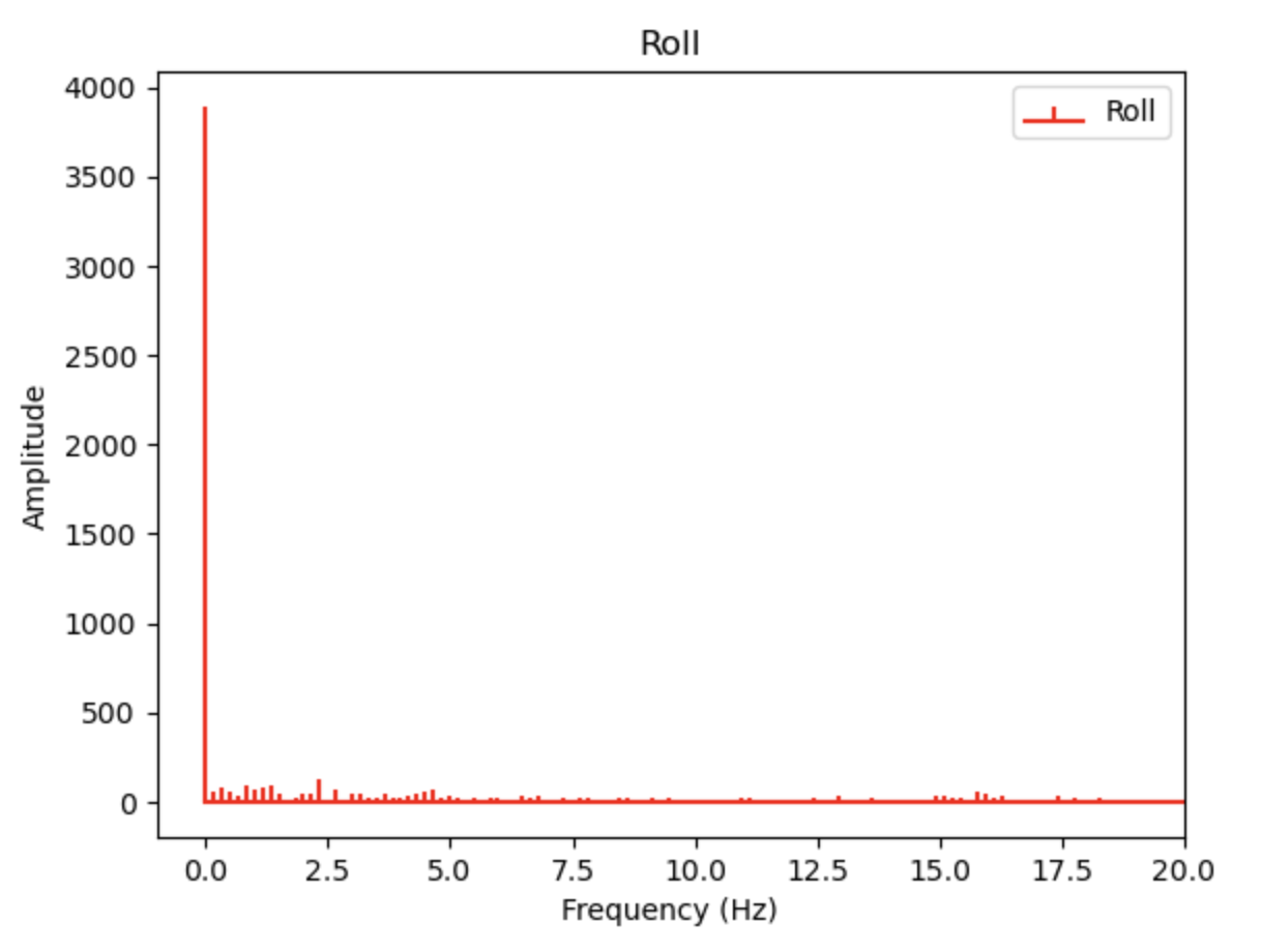
This data can be analyzed to determine its frequency components by computing a fourier transform of it. The following data are the frequency components of the pitch and roll.
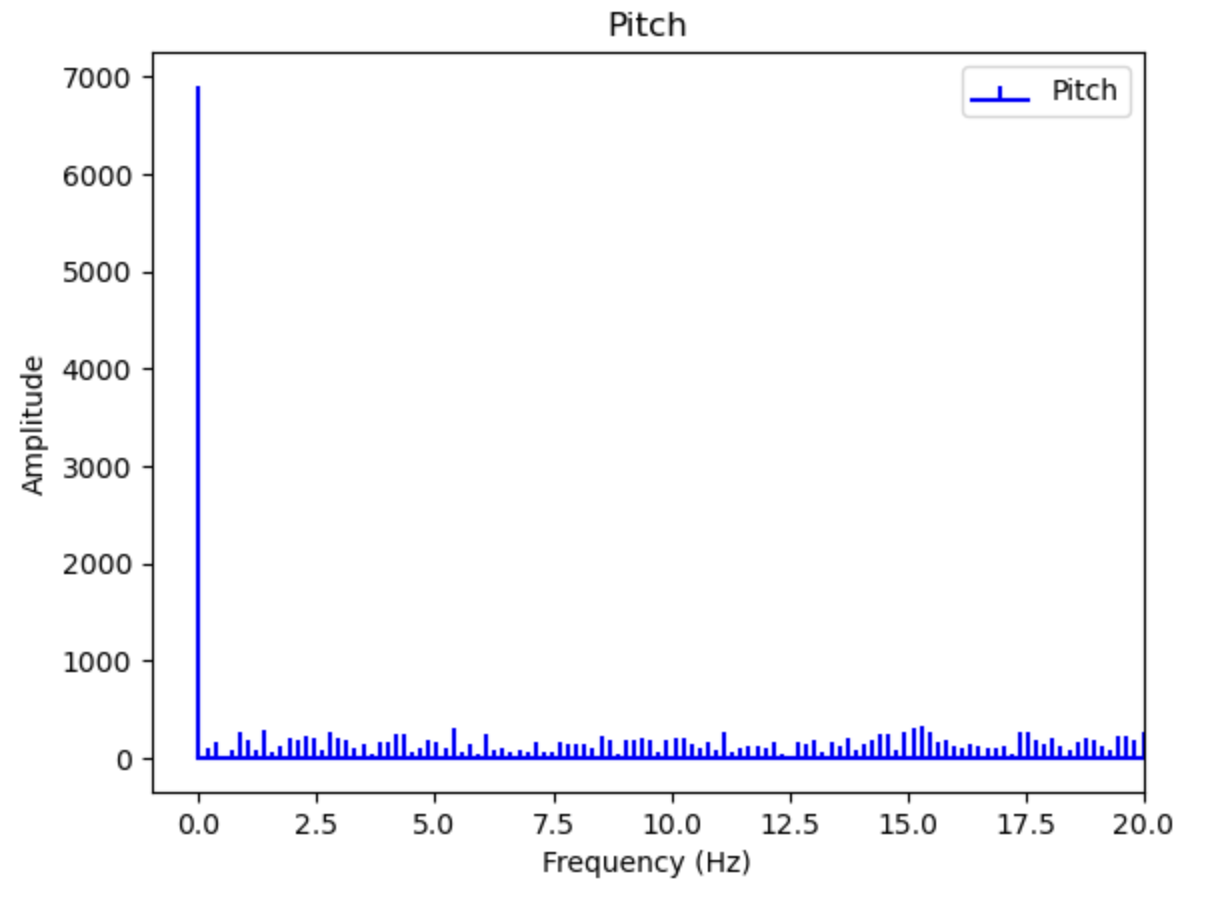
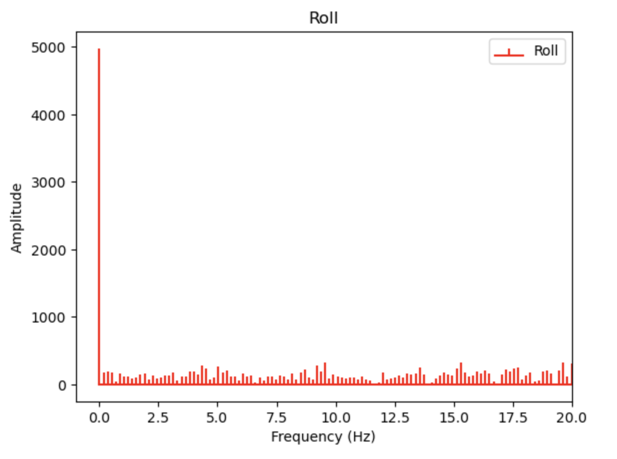
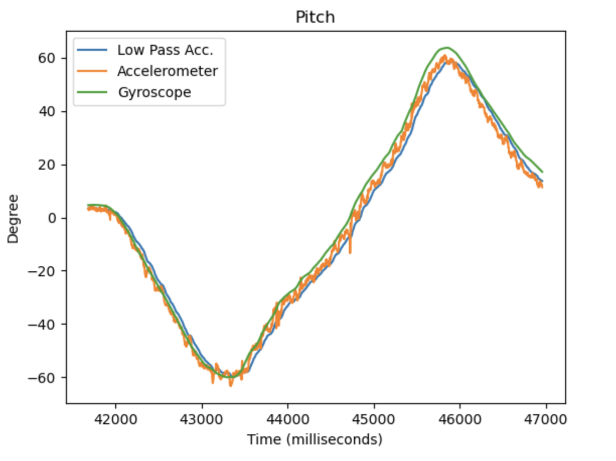
As it can be seen from the graphs, the measurements have non-zero frequency components for a large range of frequencies. This is undesirable and leads to the type of noisy data we are seeing. Therefore, I built a low-pass filter with a cutoff of about 2.5 Hz for the accelerometer data. By using such a low cut off frequency, the output of this filter is much less noisy, as can be seen below.
This slightly stabilizes the values of the pitch and roll, though they are still noisy. A complementary filter might be able to reduce this noise even more, and to implement one I will need data from the gyroscope within the IMU as well.
Gyroscope
Roll and Pitch as Determined by the Gyroscope
The gyroscope returns the angular velocity, in degrees per second, of one of the three axes of the IMU. To use this data, you must multiply the angular velocity by the amount of time since the sensor’s last sample. This returns a change in degree over some axis. If you continuously sum these changes over time you will get a very stable approximation for the pitch, roll, and yaw of the IMU.
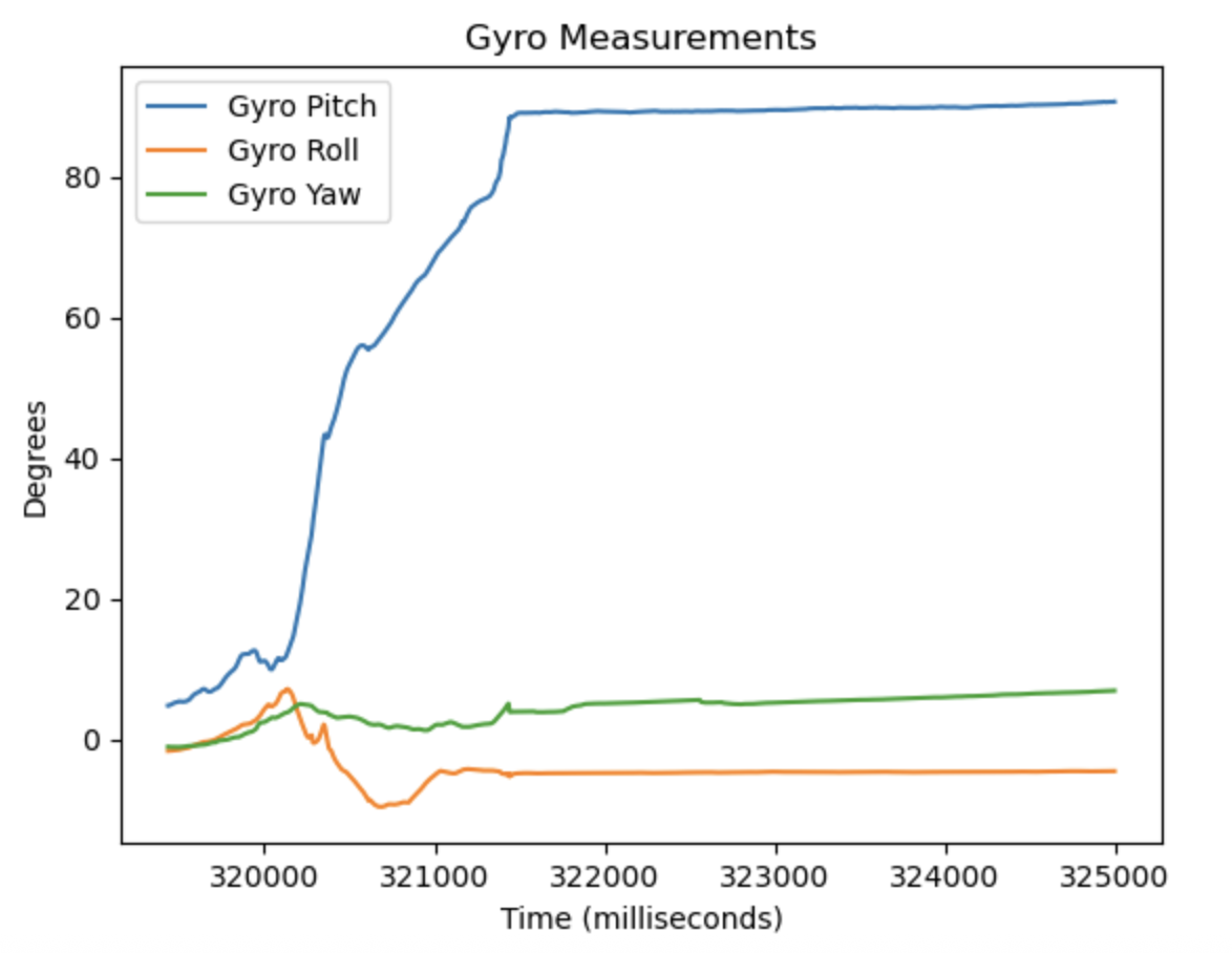
However, though the gyroscope readings have very little noise, they will drift away from the true values. This is when calculating the pitch, roll, or yaw, you continuously add upon previous measurements, summing the errors of each measurement. An example of this drift can be seen below, where though the IMU was motionless on a table, some of the angle measurements diverge from zero.
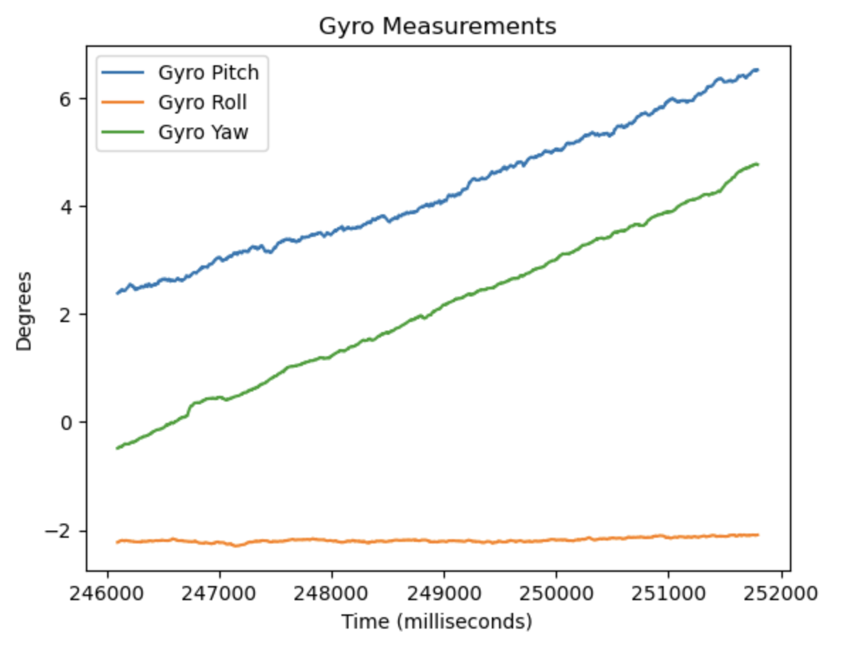
Even with this drift, the stability of the gyroscope data is very desirable. Take the following data, for example. When the IMU is moving, the gyroscope data is not noisy, resulting in a very clear calculation of the pitch, roll, and yaw of the IMU.
So far, we have the raw acceleration data, the low-passed acceleration data, and the gyroscope data to calculate the pitch and roll.
But both the accelerometer and the gyroscope have benefits and costs to their usage, so we need to implement a way to combine their data and get the best of both options.
Complementary Filter
A complementary filter must be built in order to fuse the accuracy of the accelerometer with the stability of the gyroscope. What the complementary filter will do is sum a scaled value of the accelerometer’s pitch and roll, as determined by the low-pass filter, with the pitch and roll from the gyroscope data. The question then becomes how to weigh the two sources properly.
The desirable trait of the accelerometer is that it is very accurate, but it is also very noisy. Additionally, due to the math behind the pitch and roll calculations, when either of those angles are at ±90 degrees, the other angle will behave as if at a singularity. Therefore, we would want the complementary filter to reduce the noise and remove the singularity from the data, but keep the accuracy. From the gyroscope, the complementary should remove the drift but keep the stability.
Therefore, the complementary filter should weigh the gyroscope much higher than the accelerometer. This is because by weighing the gyroscope data higher, the complementary filter will prioritize stability and non-singularity behavior more on shorter time scales. The smaller component of the accelerometer data will not change the output of the filter from one time step to another, but over long time scales the accelerometer’s contribution will help to compensate for the drift of the gyroscope and will bring the filter back to an accurate value of the pitch and roll. This will produce a system that will have the same accuracy as the accelerometer, but have the non-singularity filled range of the gyroscope.
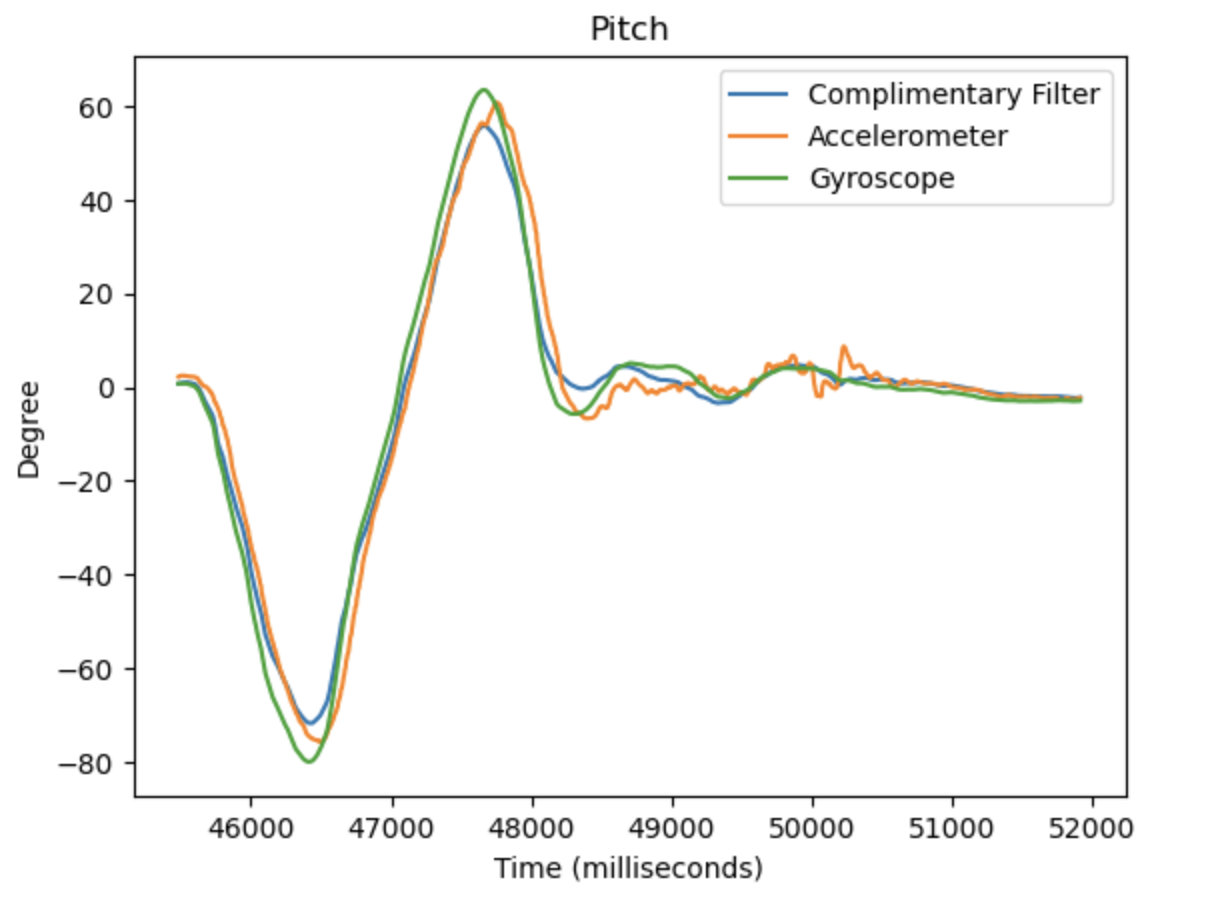
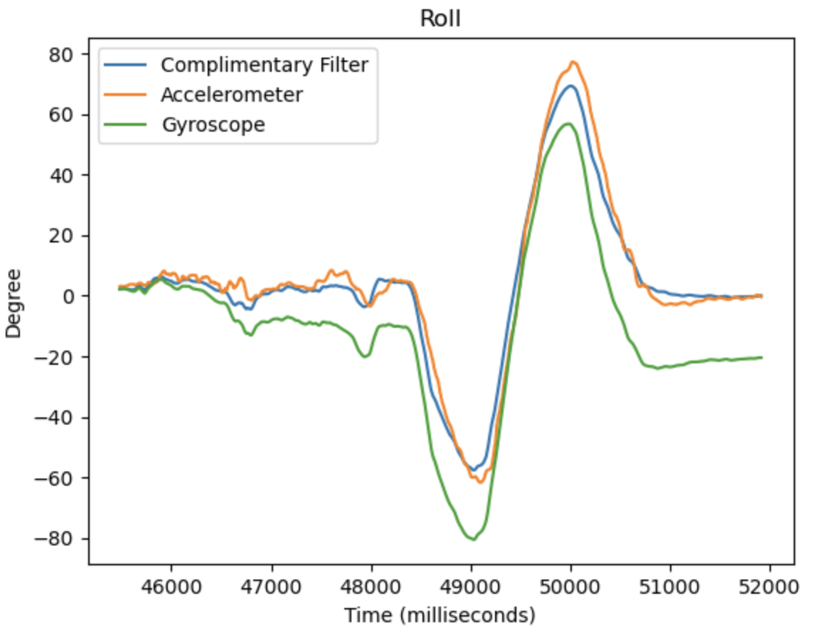
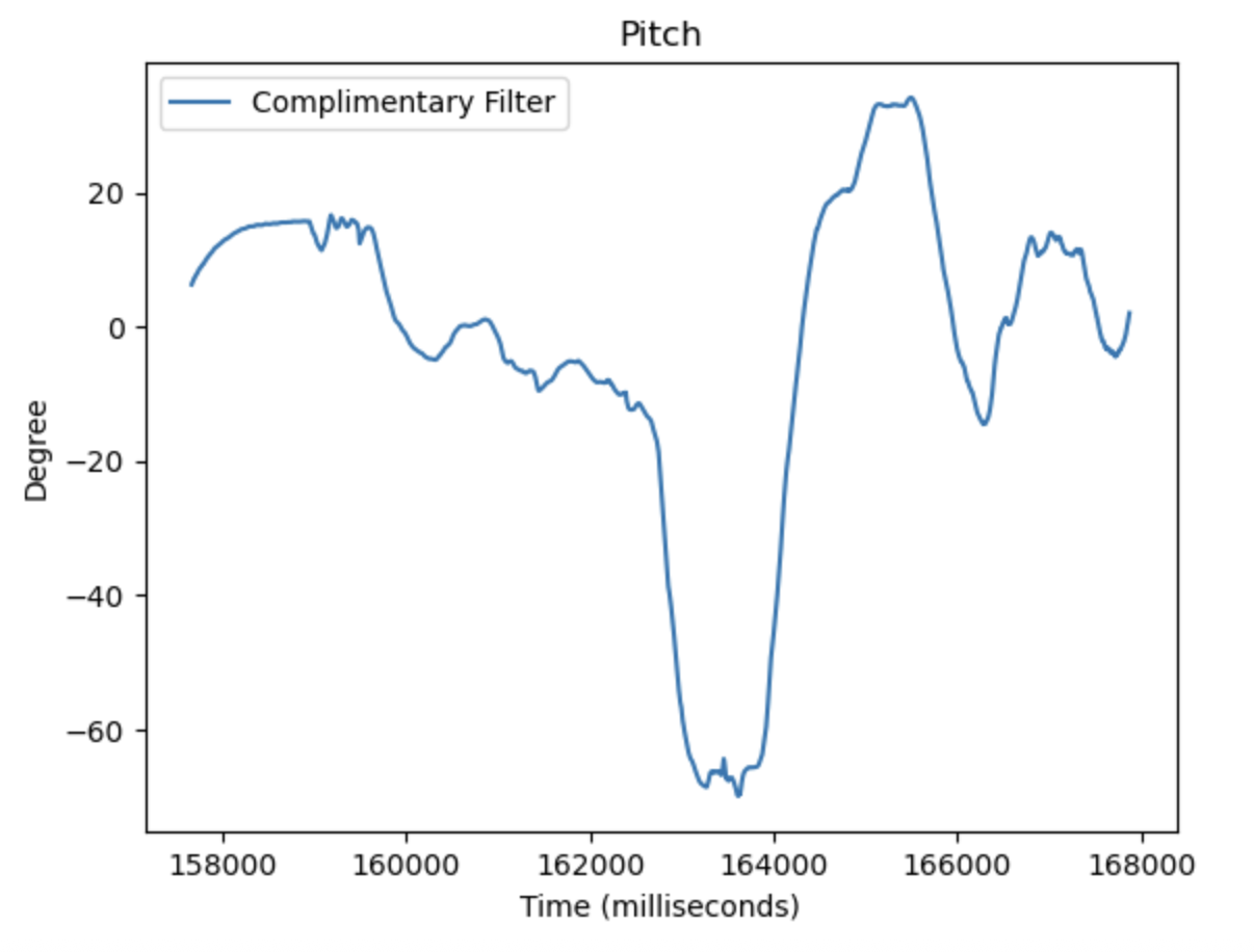
After various attempts, I decided that weighting the gyroscope data with 0.99 and the accelerometer data with 0.01 was best. This can be seen in the first image below when the complementary filter isn’t affected by the low-pass accelerometer’s odd noise at around 50000 milliseconds, time step. In the second image, the complementary filter follows the same shape as the gyroscope, and is non-noisy, but the accelerometer data brings the filter’s output back to an accurate value.
Sampling Data
Collection and Storage of Time-Stamped IMU Data
In order to achieve the highest rates of data transfer possible, I collected the data in arrays on the Artemis Nano, filling the arrays entirely before sending any data over Bluetooth to my laptop. This was done in Arduino by looping over the arrays of fixed size and updating their entries. For example:
time_array[counter] = (int)millis();

...

theta_filter_rad[counter] = (theta_filter_rad[counter-1] - dy)*(1.0-alpha_complimentary_filter)+(((theta_a*180)/M_PI)*alpha_complimentary_filter);
phi_filter_rad[counter] = (phi_filter_rad[counter-1] + dx)*(1.0-alpha_complimentary_filter)+(((phi_a*180)/M_PI)*alpha_complimentary_filter);
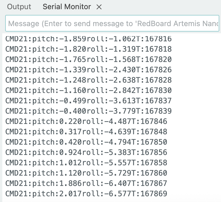
The above code looped through the lists, incrementing counter until it reached the length of the list. At this point, the entire list of data was transmitted to my laptop and printed to the Arduino serial monitor one index at a time. Below is how this data was organized for transmission. The “CMD21:” section of the data was used on the Python end of the system in order for it to determine what data was sent with this associated command.
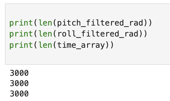
The arrays storing the pitch, roll, and time values were 3000 indices long, and all of these data were stored in lists in Python on my laptop after being transmitted by the Artemis Nano.
I believe that it makes most sense to store the pitch, roll, and time data in separate arrays of floats and integers. This decreases any additional memory required to store an array of specialized structs. It is not more memory efficient to store all of the data into one large array because you would have to cast all the data to the same type of variable, which can actually increase memory usage. Additionally, storing all of the data in one large array would become harder for the Python scripts to sift through and use, adding to the computational complexity of analyzing the sensor’s readings.
As discussed in Lab 1, the amount of memory that I can allocate to my arrays depends on the number of arrays that I have. If, for example, I only care about the pitch and roll output from the complementary filter and the time, then I would only need three arrays. Two of these arrays would be of floats, and the time associated array would be made of integers. This means that to store one element in each of these three arrays will collectively cost 12 bytes of memory, because both floats and integers are 4 bytes. Given that there are 384 kB of RAM, there is an upper limit of 32 kB per array available. However, this is purely a theoretical uper limit and would most likely not be true in any real system because other parts of the program may also be stored in RAM. It might be more safe to say that we could allocate half of that value to the arrays, so 16 kB per array.
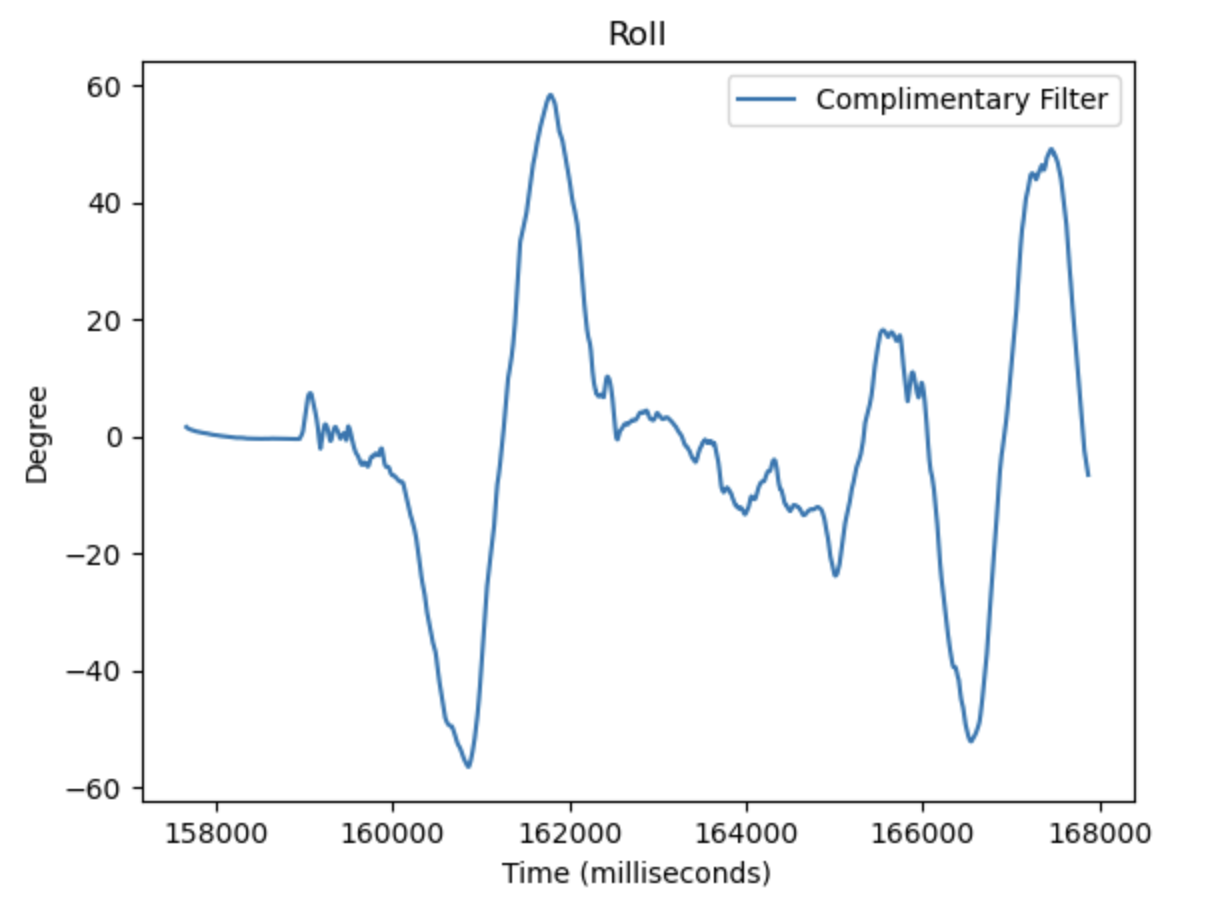
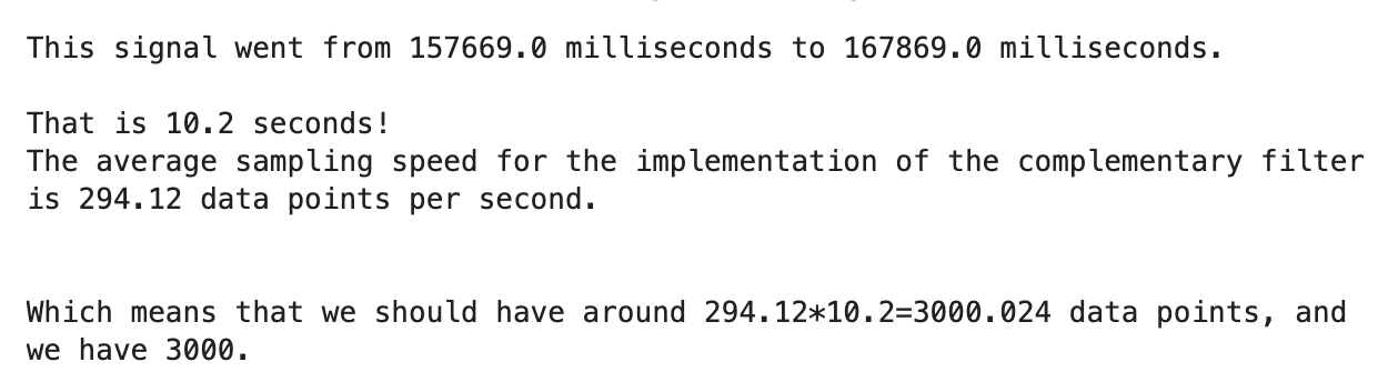
Duration of IMU Data Collection
In order to ensure that the robotic system will have enough data to work with at a time, it is helpful to have data be collected for large amounts of time. I was able to get my system to collect data for more than 10 seconds at frequency of about 294 data points per second, as shown below.
Record a Stunt
The car is very responsive and fast. It is able to change directions quickly, as well as flip over when changing direction. The button on the top left of the remote seems to make the car “go crazy”, making it move and flip around. It is a little bit difficult to turn the car accurately. Similarly, it was hard to turn while moving, often resulting in chaotic motions.