Lab 12: Inverted Pendulum

For the final lab of this course, students had the option of either navigating the built environment that we performed mapping and Bayes filtering on previously, or to implement an inverted pendulum stunt with the car. Because I am more interested in controls than mapping or navigation, I decided to attempt to implement the inverted pendulum stunt. For this stunt, I needed to stabilize the motion of the car while also attempting to balance one side of the car directly above the other side, an inherently very unstable position to put a car into.

Control Logic

In order to control the car, I decided to use a linear quadratic regulator (LQR) to determine what control gains would be needed to optimally maintain the car’s upright position. To do this, I needed to model the system dynamics of the car, linearize this model about the point of interest, discretize the continuous model, and then finally use Python to solve the Ricatti Equation to derive the optimal gain K.

Lagrangian Background

To develop a mathematical model of the car’s dynamics, it is necessary to start from a force balance equation and work backwards from there to see how the input affects the various states of the car. This, however, can be quite difficult for complex systems, and it is easier to use Lagrangian Mechanics as opposed to Newtonian Mechanics.

Lagrangian Mechanics states that the lagrangian, $L$, is equal to the kinetic energy $K$ minus the potential energy $P$.

\[L = K - P\]

Once we know $L$, we can use the following relationship to determine how the inputs into the system affect its states:

\[\frac{d}{dt}(\frac{\partial L}{\partial\dot{q}_i}) - \frac{\partial L}{\partial q_i} = Q_i\]

Where $q_i$ represents one of the states of the system, and $Q_i$ represents the force affecting the state $q_i$. To use this, therefore, we need to determine what $K$ and $P$ are.

Mathematical Model

I will use the following diagram (borrowed from lecture material) to represent the inverted pendulum system. The only change I will make is that the offset of $\pi$ will be an offset of $\pi/2$ in my system.

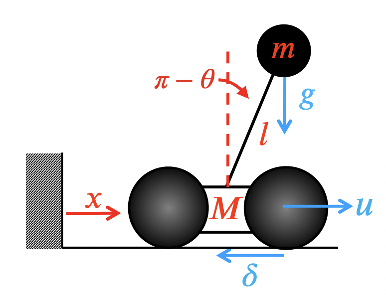
Here, $M$ is the mass of the lower portion of the pendulum, $m$ is the mass of the upper portion, $l$ is the length between them, $\delta$ represents friction, $u$ is the PWM input into the bottom wheels, $\theta$ is the pitch of the car relative to the ground, and $x$ is its distance from a wall.

From this, we have the following state representation.

\[y = \begin{bmatrix} x \\ \dot{x} \\ \theta \\ \dot{\theta} \end{bmatrix}\]

From this, we can derive equations for both $P$ and $K$:

\[P = -mgl\cos\theta\] \[K = \frac{1}{2}(M+m)\dot{x}^2 + \frac{1}{2}ml^2\dot{\theta}^2-m\dot{x}\dot{\theta}l\sin\theta\]

This results in:

\[L = K-P = \frac{1}{2}(M+m)\dot{x}^2 + \frac{1}{2}ml^2\dot{\theta}^2 - m\dot{x}\dot{\theta}l\sin\theta - mgl\sin\theta\]

For $q_1 = x$, we have the following:

\[Q_1 = F - \delta\dot{x}\] \[\frac{\partial L}{\partial x} = 0\] \[\frac{\partial L}{\partial \dot{x}} = (M+m)\dot{x} - m\dot{\theta}l\sin\theta\] \[\frac{d}{dt}(\frac{\partial L}{\partial \dot{x}}) = (M+m)\ddot{x} - m\ddot{\theta}l\sin\theta - m\dot{\theta}^2l\cos\theta\]

Resulting in:

\[(M+m)\ddot{x} - m\ddot{\theta}l\sin\theta - m\dot{\theta}^2l\cos\theta = F - \delta\dot{x}\]

For $q_2 = \theta$, we have the following:

\[Q_2 = 0\] \[\frac{\partial L}{\partial \theta} = -m\dot{x}\dot{\theta}l\cos\theta - mgl\cos\theta\] \[\frac{\partial L}{\partial \dot{\theta}} = ml^2\dot{\theta} - m\dot{x}l\sin\theta\] \[\frac{d}{dt}(\frac{\partial L}{\partial \dot{\theta}}) = ml^2\ddot{\theta} - m\ddot{x}l\sin\theta - m\dot{x}\dot{\theta}l\cos\theta\]

Resulting in:

\[ml^2\ddot{\theta} - m\ddot{x}l\sin\theta + mgl\cos\theta = 0\]

Combining the computed terms allows us to create the following matrix equation:

\[\begin{bmatrix} (M+m) & -ml\sin\theta \\ -ml\sin\theta & ml^2 \end{bmatrix} \begin{bmatrix} \ddot{x} \\ \ddot{\theta} \end{bmatrix}= \begin{bmatrix} F - \delta\dot{x} + m\dot{\theta}^2l\cos\theta \\ -mgl\cos\theta \end{bmatrix}\]

Solving the above equation for $\left[ \ddot{x},\ \ddot{\theta} \right]^T$ results in the following matrix, where $\Delta = ml^2(M+m(1-\sin^2\theta))$.

\[\begin{bmatrix} \ddot{x} \\ \ddot{\theta} \end{bmatrix}= \begin{bmatrix} \frac{ml^2(F - \delta\dot{x} + m\dot{\theta}^2l\cos\theta - mg\sin\theta\cos\theta)}{\Delta} \\ \frac{ml\sin\theta(F - \delta\dot{x} + m\dot{\theta}^2l\cos\theta) - (M+m)(mgl\cos\theta)}{\Delta} \end{bmatrix}\]

From here, we get:

\[\frac{d}{dt} \begin{bmatrix} x \\ \dot{x} \\ \theta \\ \dot{\theta} \end{bmatrix}= \begin{bmatrix} \dot{x} \\ \frac{ml^2(F - \delta\dot{x} + m\dot{\theta}^2l\cos\theta - mg\sin\theta\cos\theta)}{\Delta} \\ \dot{\theta} \\ \frac{ml\sin\theta(F - \delta\dot{x} + m\dot{\theta}^2l\cos\theta) - (M+m)(mgl\cos\theta)}{\Delta} \end{bmatrix}\]

Model Linearization

With the above matrix representation in hand, we can now linearize if about $x=free$, $\dot{x}=0$, $\theta=\pi/2$, and $\dot{\theta}=0$. After a lot of math, this eventually outputs:

\[\frac{d}{dt} \begin{bmatrix} x \\ \dot{x} \\ \theta \\ \dot{\theta} \end{bmatrix}= \begin{bmatrix} 0 & 1 & 0 & 0 \\ 0 & -\frac{\delta}{M} & \frac{mg}{M} & 0 \\ 0 & 0 & 0 & 1 \\ 0 & -\frac{\delta}{Ml} & \frac{g(M+m)}{Ml} & 0 \end{bmatrix} \begin{bmatrix} x \\ \dot{x} \\ \theta \\ \dot{\theta} \end{bmatrix} + \begin{bmatrix} 0 \\ \frac{1}{M} \\ 0 \\ \frac{1}{Ml} \end{bmatrix} F\]

This, however, includes information of $x$ and $\dot{x}$, which I am not actually interested, so it can be reduced to the following form:

One remaining issue is that we can input PWM signals to the motors of the car, and I am unsure of how this maps to a force $F$. The force applied by the wheel will be equal to the wheel’s torque divided by its radius, $\frac{\tau}{r}$, and I know that $\tau$ will be proportional to $u$ by some scaling factor $\alpha$ such that $F = \frac{\tau}{r} = \frac{\alpha u}{r}$. With this, we can rewrite the above expression to finally get:

\[\begin{bmatrix} \dot{\theta} \\ \ddot{\theta} \end{bmatrix}= \begin{bmatrix} 0 & 1 \\ \frac{g(M+m)}{Ml} & 0 \end{bmatrix} \begin{bmatrix} \theta \\ \dot{\theta} \end{bmatrix} + \begin{bmatrix} 0 \\ \frac{\alpha}{Mlr} \end{bmatrix} u\] \[A= \begin{bmatrix} 0 & 1 \\ \frac{g(M+m)}{Ml} & 0 \end{bmatrix}\] \[B= \begin{bmatrix} 0 \\ \frac{\alpha}{Mlr} \end{bmatrix}\] \[\begin{bmatrix} \dot{\theta} \\ \ddot{\theta} \end{bmatrix}= A \begin{bmatrix} \theta \\ \dot{\theta} \end{bmatrix}+ Bu\] \[\dot{y}= Ay + Bu\]

With this state dynamics representation in continuous time, we can now discretize $A$ and $B$ because the actual car updates in discrete time.

Model Discretization and Python Implementation

I decided to discretize the system with $dt = 0.006148$ seconds, which was the average period of time that my control loop for the inverted pendulum stunt performed at. To discretize $A$, one must compute $e^{Adt} = A_d$. To discretize $B$, one needs to calculate $(\int_{0}^{dt} e^{A\tau} \,d\tau)B$. Luckily, when $A$ is invertible, this reduces to $B_d=A^{-1}(A_d-I)B$. In Python this looked like:

A_cont = np.array([[0, 1], [(g*(M+m))/(M*l), 0]])
B_cont = np.array([[0], [alpha/(M*l*r)]])

A_dis = expm(A_cont*dt)
B_dis = np.linalg.inv(A_cont) @ (A_dis - np.eye(2)) @ B_cont

I was able to determine some of the characteristics of the system by directly measuring it. For example, using a caliper I found $l = 0.10195 [m]$ and $r = 0.04081 [m]$. I was able to find the total weight of the car, $M+m = 0.532 [kg]$, but I wasn’t sure how large $M$ was compared to $m$. Additionally, I wasn’t exactly sure how the PWM input scaled to torque output, so $\alpha$ was unknown. Therefore, both of these characteristics became things that I needed to tune when testing the LQR output.

g = 9.81 # m/s^2
total_car_mass = 0.532 # kg
fraction_of_top = 0.4 # a guess
fraction_of_bottom = 1 - fraction_of_top
m = fraction_of_top*total_car_mass # kg
M = fraction_of_bottom*total_car_mass # kg
l = 0.10195 # m
r = 0.04081 # m 
alpha = 0.065/255 # Nm/pwm, a guess
dt = 0.006148 # seconds

The LQR output is called the LQR gain $K$, and it allows a system to find the optimal control given its current state by $u = -Ky$, where $y=\left[ \ddot{x},\ \ddot{\theta} \right]^T$. To find this, it is also necessary to define the $Q$ and $R$ matrices. $Q$ represents how much you care that either state is at its set point, and $R$ represents how much you care about the input cost of getting to the set point. In the inverted pendulum system, I care heavily that $\theta=90$ degrees, and less importantly that $\dot{\theta}=0$. Since I am just trying to stabilize the system and I don’t care about how much effort it takes to do it, I can set $R$ relatively low, shifting the focus of the LQR to prioritize the proper orientation and speed instead. For all my trials I have $R=[[0.001]]$. Tuning the value of $Q$ is a part of any LQR, and for my system I must also tune $\alpha$ and the computational representation of the distribution of mass.

After $Q$ and $R$ are defined, finding $K$ is easy.

Q = np.array([[250, 0], [0, 100]])
R = np.array([[0.001]])

X = solve_discrete_are(A_dis, B_dis, Q, R)

K = (np.linalg.inv(R+B_dis.T@X@B_dis))@(B_dis.T@X@A_dis)

I can then send the values of the computed LQR gain to the Artemis to use for its control loop via a Bluetooth command.

k0 = round(K[0][0],2)
k1 = round(K[0][1],2)

string = str(k0) + "|" + str(k1)

ble.send_command(CMD.SET_LQR_GAINS, string)

I also make it so that I can start and stop the controller from running on the Artemis, which was helpful when I wanted to try new LQR gain values.

ble.send_command(CMD.START_INVERTED_PENDULUM, "")

ble.send_command(CMD.STOP_INVERTED_PENDULUM, "")

Control Implementation

The control loop in the Artemis was essentially a PD controller, with kp and kd being determined by the first and second value of the LQR gain $K$. For the error, I used the difference between a low-passed filtered pitch calculation from the accelerometer data. I did not think that it was necessary to build a full Kalman Filter for pitch estimation since the IMU sampling rate was relatively fast, especially since I removed the DMP initialization and usage for this stunt in particular. For the derivative term, I took the derivative of the pitch as opposed to the derivative of the error by simply using the gyroscope reading.

I made sure to account for any offset the accelerometer might report due to a slight tilt in its placement on the car which may have not been visible to me. This, as well as calculating a gyroscope bias, is done in the first if statement in the function that I built, inverted_pendulum(). After that, this calibration is never run again and a simple control loop takes place. I calculate the pitch, find the error from the desired pitch minus any unintentional offset, determine the angular speed, use the gains from the LQR, and determine the PWM output to the motors.

I also track pitch, PWM input, and timing data, which I return to my laptop via Bluetooth once STOP_INVERTED_PENDULUM is called.

The following is the final version of my control function:

void inverted_pendulum(){

   drive_motors(pwm_input);

   if (first_run_pendulum) {

       int place_holder = 0;
       while (place_holder < 500){
           if (myICM.dataReady()){
               myICM.getAGMT();
               gyro_bias = gyro_bias + myICM.gyrX();
               delay(2);
               place_holder = place_holder + 1;
           }
       }

       gyro_bias = gyro_bias/500;

       while (!first_data_collected){
           if (myICM.dataReady()){
               acc_x = myICM.accX();
               acc_y = myICM.accY();
               acc_z = myICM.accZ();
               gyro_x =myICM.gyrX() - gyro_bias;
               first_data_collected = 1;
           }
       }

       angular_speed = (gyro_x*PI)/180.0;
       acc_pitch = atan2(acc_y, acc_z);
       pitch = acc_pitch;
       pitch_offset = pitch;

       first_run_pendulum = 0;

       previous_time = micros();

   } else {
       if (myICM.dataReady()){
           myICM.getAGMT();
         
           acc_y = (1-a_y)*myICM.accY()+(a_y*acc_y);
           acc_z = (1-a_z)*myICM.accZ()+(a_z*acc_z);
           gyro_x = myICM.gyrX()-gyro_bias;

           acc_pitch = atan2(acc_y, acc_z);
           angular_speed = (gyro_x*PI)/180.0;

           current_time = micros();
           dt_pendulum = ((float)(current_time - previous_time))*1e-6;
           previous_time = current_time;

           pitch = 0.9*pitch + 0.1*acc_pitch;
           pitch_error = (-PI/2 - pitch_offset) - pitch;

           input = -1*(k0*pitch_error - k1*angular_speed);
           pwm_input = input;

           if ((abs(pitch_error) >= cutoff_radians)) {
               pwm_input = 0;
           } else {
               if (pwm_input >= 0){
                   if (pwm_input > 255){
                       pwm_input = 255;
                   }
               } else {
                   if (pwm_input < -255){
                       pwm_input = -255;
                   }
               }
           }

           if ( dt_counter < length_of_array ){
               yaw1[dt_counter] = pitch;
               pwm[dt_counter] = pwm_input;
               time_array[dt_counter] = current_time;
               dt_counter = dt_counter + 1;
           }
       }
   }
}

Real System Behavior and Tuning

Initially, I had the goal pitch as 90°. My first attempt at this was relatively poor, as can be seen in the video below.

One of the next trials I conducted had $Q=[[250,0],[0,100]]$, $\alpha=\frac{0.07}{255}$, and 40% of the mass of the car at the top of the inverted pendulum. This resulted in LQR gains of k0 = 1519.93 and k1 = 279.95. These gains produced the following output.

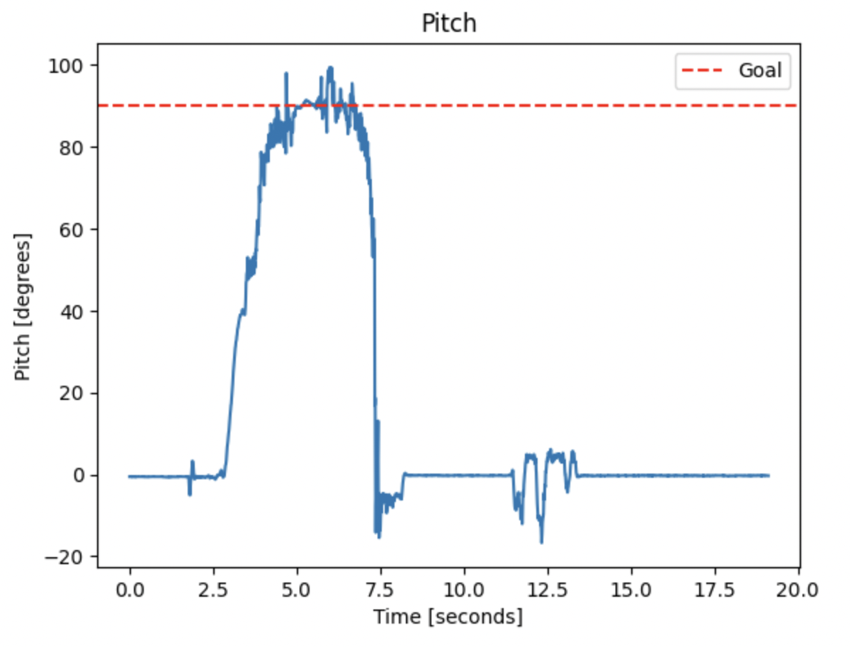
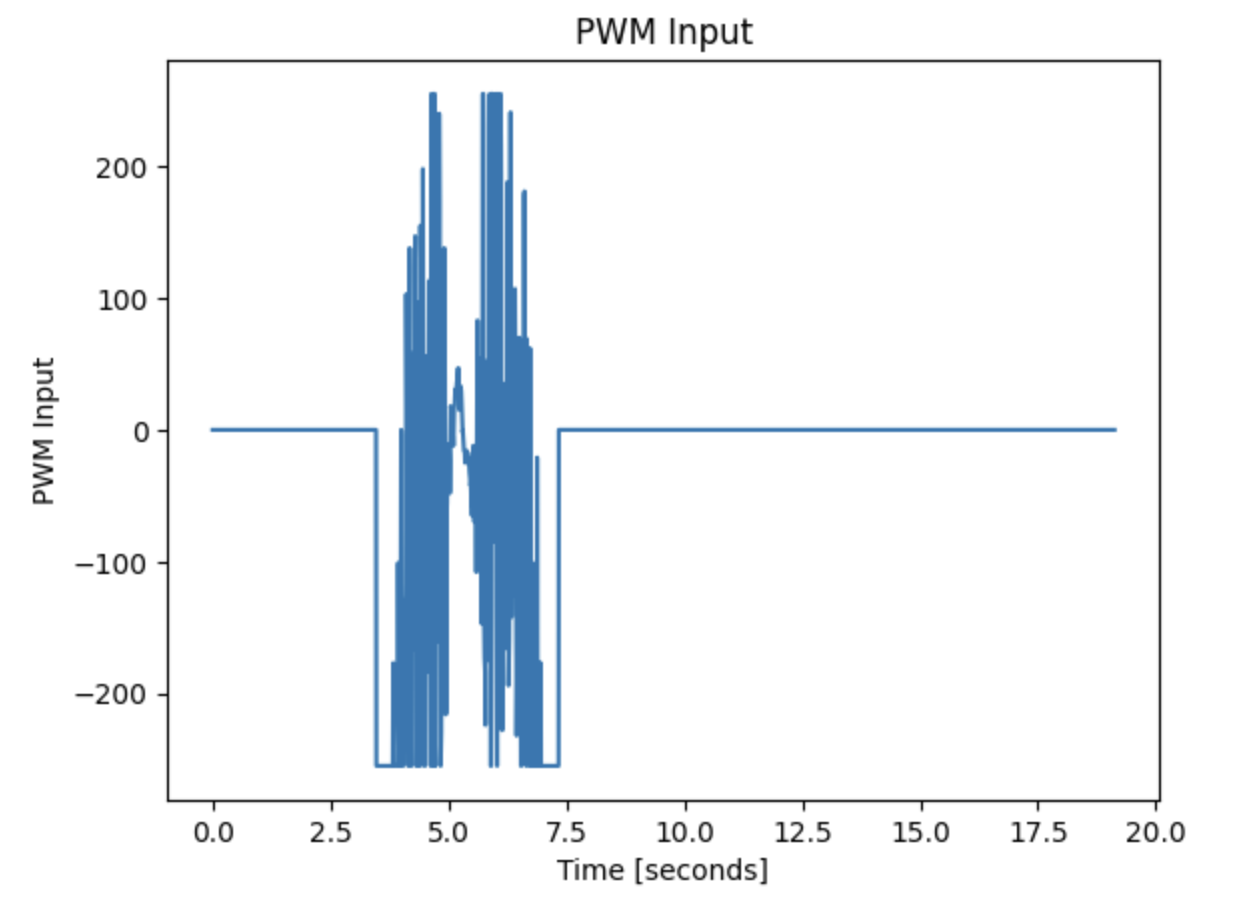
I won’t include all of my trials, but it is interesting to note that the most ideal controller gains I found corresponded with almost the exact same setup as the trial shown above. The only difference was changing $\alpha$ to $\frac{0.065}{255}$, a minor difference of 0.0000196 from the previous value.

The biggest change wasn’t with my parameters, it was with my physical setup. After hours of watching the car destabilize and fall, I accidentally flipped the car the opposite way. Instead of a pitch of 90°, I moved it to -90°. I didn’t notice the mistake, but the results were clear. The car was actually stabilizing and not just falling over!

This trial is shown below, along with the data from that trial.

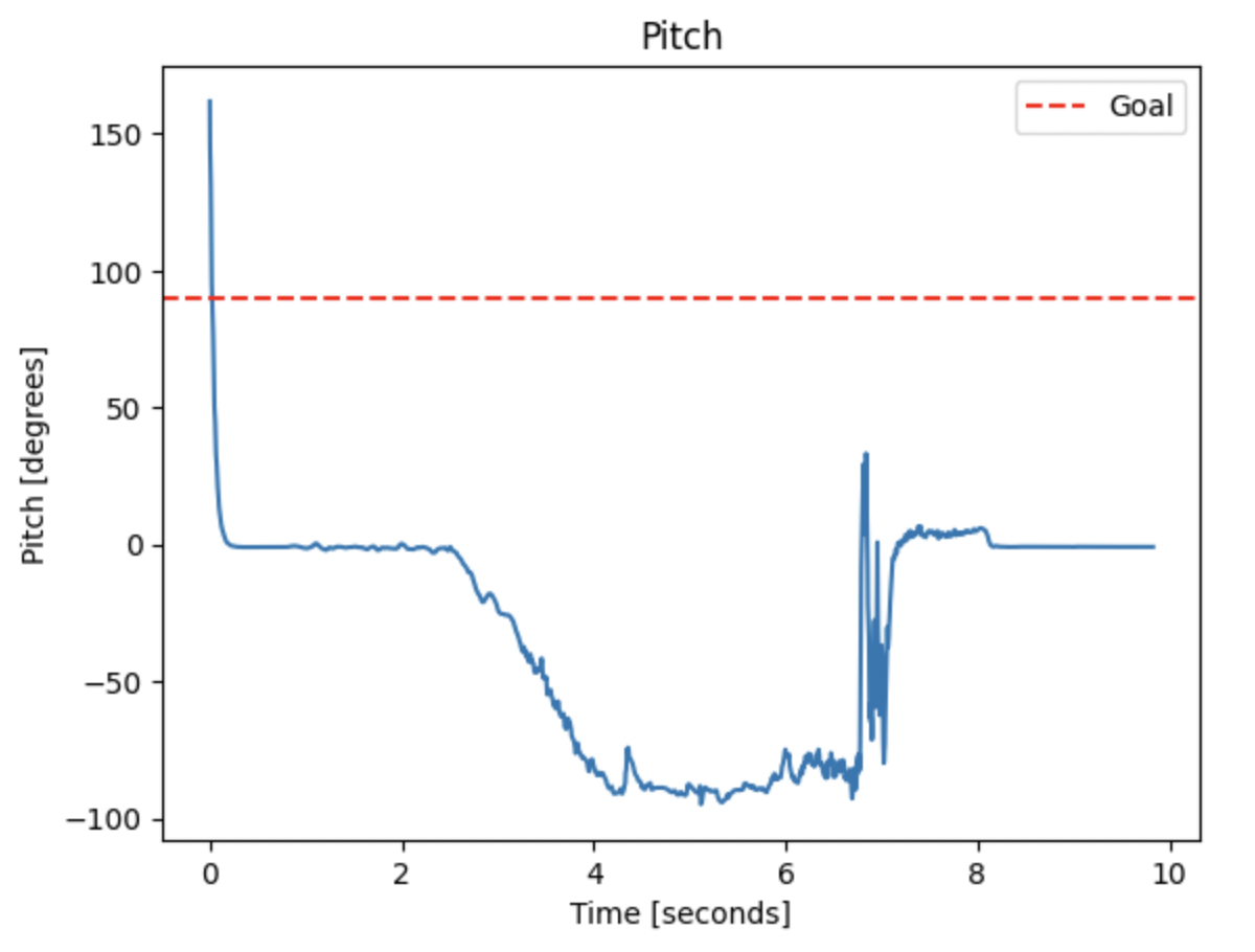
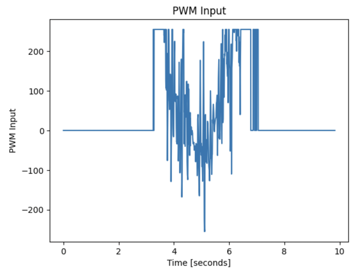
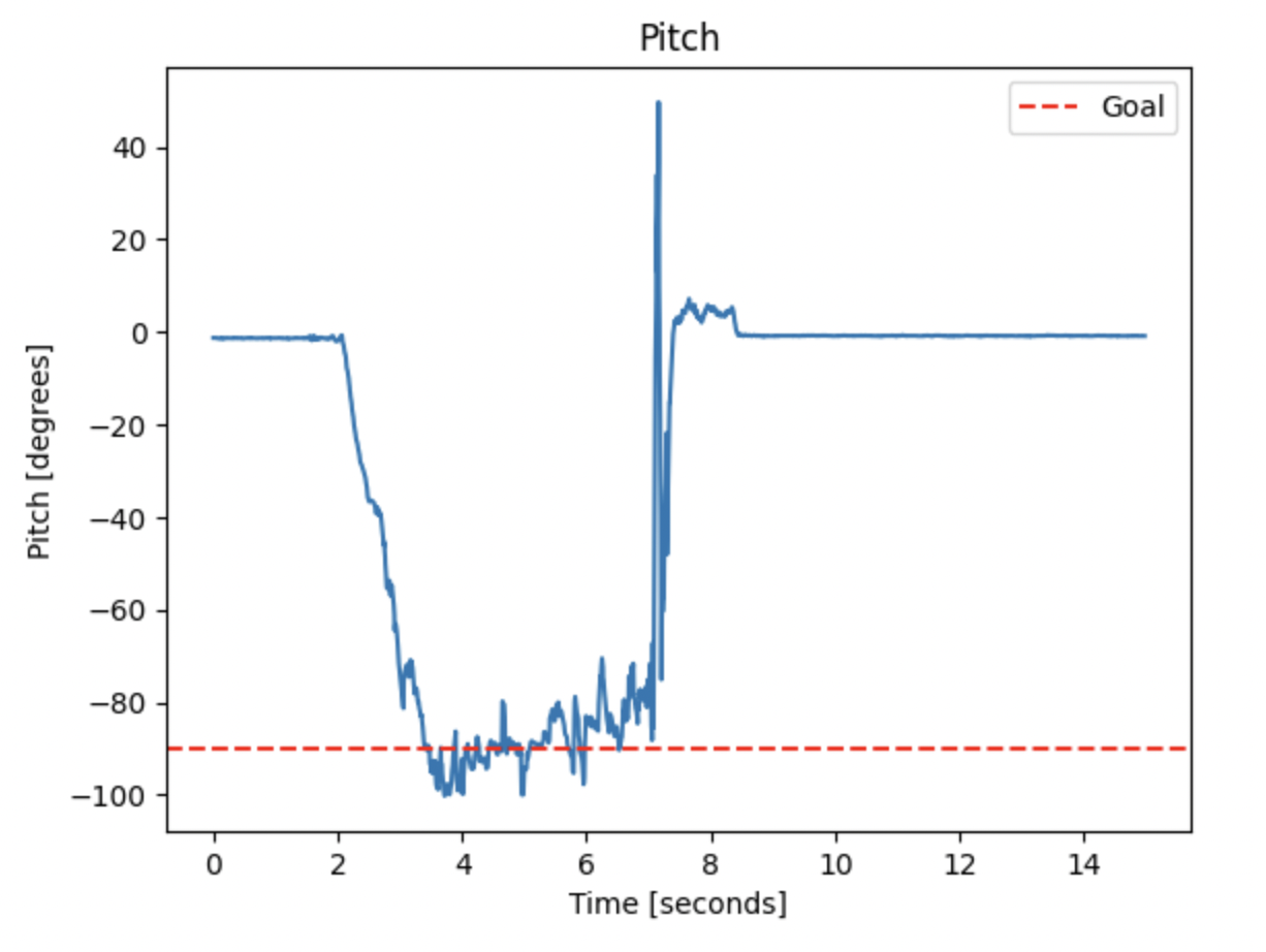
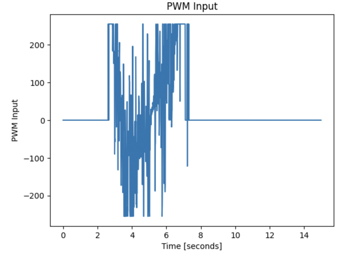
To reiterate, the two previous trials were run with almost identical LQR gains. The only significant difference was the orientation of the car. I assume that this is because when I accidentally flipped the car, the IMU was at the top of the pendulum instead of at the base. This could theoretically allow the IMU to more quickly relay accurate pitch and angular velocity data about the top of the inverted pendulum as compared to when it was positioned at the bottom. This allowed for the control loop to react faster, causing the car to stabilize.

After making this realization, I changed the control loop code so that the setpoint was -90°, and ran the following trial.

Conclusion and Acknowledgements

The gain from an LQR works great, but only if your actual system matches the representation used in the math of the LQR. Make sure to always double check this to save yourself time and effort! I referenced Stephan Wagner’s and Nita Kattimani’s previous course websites when completing this lab.

I truly enjoyed this course, and loved working on everything from soldering hardware to mapping to controlling inherently unstable systems. My knowledge of robotics has definitely been deepened, and I can’t wait to use what I have learned in the future!

ECE 4160 Fast Robots

Project Documentation of Lalo Esparza's ECE 4160 Labs