Lab 11: Localization on the Real Robot
In this lab, we implement the Bayes Filter on the actual robot in order to perform localization.
Using the Simulator
Before attempting to run the Bayes algorithm on the physical hardware, it was necessary to verify the credibility of the Bayes filter using the simulation software. In a process very similar to that of Lab 10, the Bayes Filter localizes the robots using an odometry motion model and a sensor model. The given Lab 11 files output the following result for localization, where green represents the true position of the robot, blue represents the belief, and the red represents the dead reckoning.
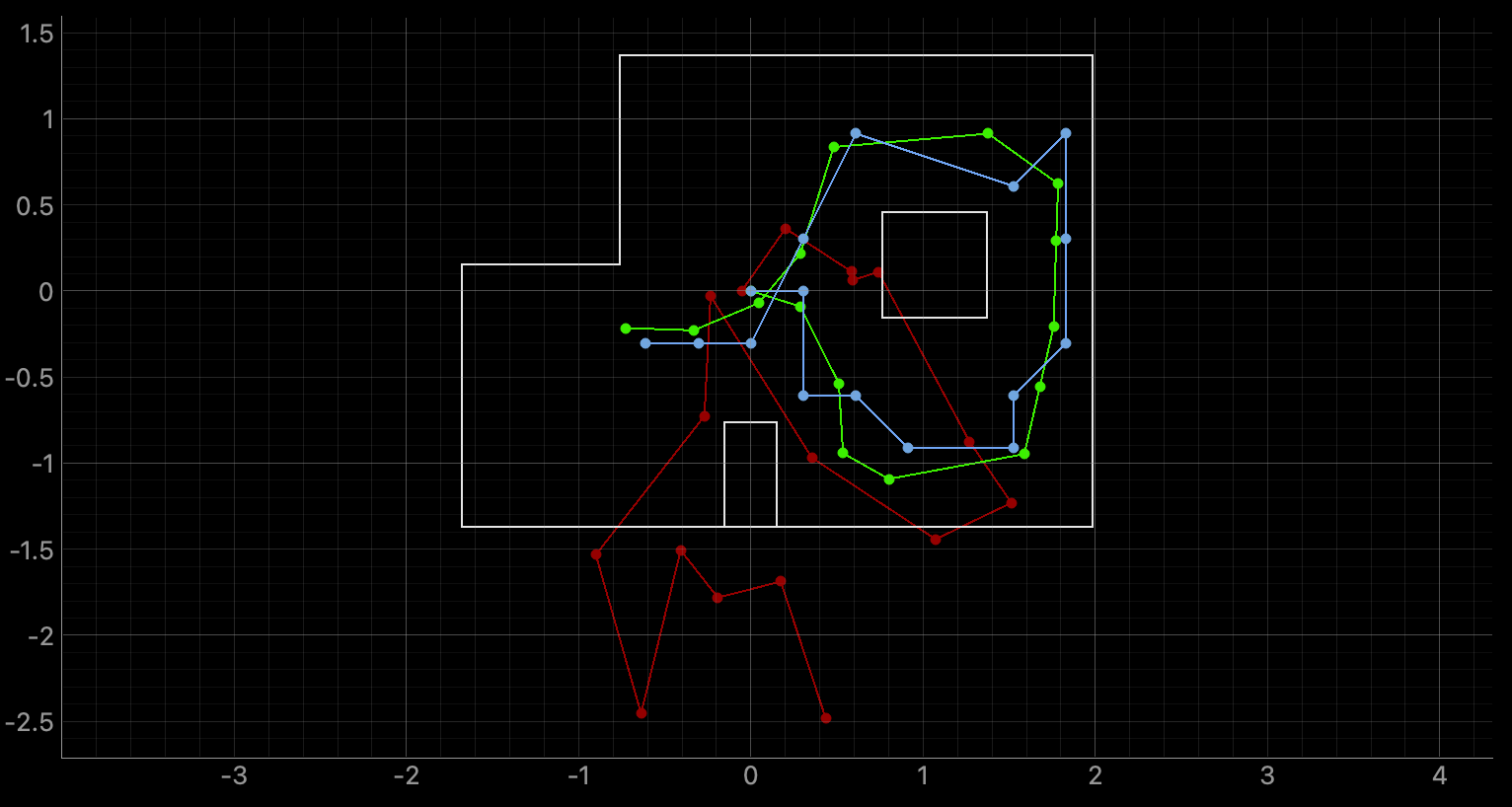
This looks like the same exact output that was found in Lab 10, indicating that the algorithm is working properly.
Physical Implementation
Now that the Bayes Filter is verified to be functional, the only component we are missing in order to localize the physical robot is the sensor data. Ideally, the robot should rotate in 20° increments, taking a measurement at each increment, totalling at 18 measurements. This matches with the number of measurements that the Bayes Filter is expecting to process, allowing us to localize the physical robot as if it was a simulated one.
Luckily, a lot of the logic for spinning in place and taking measurements was already created in Lab 9! I was able to reuse my DO_MAPPING Bluetooth command and Arduino functionality in order to have the robot take measurements at 20° increments.
The Robot Class
Initialization
Controlling the robot was handled by the given software through the use of a RealRobot class. The class originally initialized with attributes associated with the map of the world the robot is in, as well as commander and BLE objects in order to interact with both the software and hardware. I added:
        self.time = []
        self.tof0 = []
        self.tof1 = []
        self.heading = []
So that I could keep a running list of the sensor data as it came in.
Bluetooth Notifications Handler
I ran into issues when attempting to send BLE commands to the Artemis when I had defined my Bluetooth Notifications Handler outside of the class, so I decided to make it a class function.
    def start_string_notifications(self, uuid, string_notification):
        # user should always have time data returned last in arduino
        received_string = self.ble.bytearray_to_string(string_notification)
        temp_index = received_string.find("Temp:")
        time_index = received_string.find("T:")
        map_index = received_string.find("map:")
        heading_index = received_string.find("yaw:")
        tof0_index = received_string.find("tof0:")
        tof1_index = received_string.find("tof1:")

        if (map_index != -1):
            self.heading.append((received_string[heading_index + 4:tof0_index]))
            self.tof0.append((received_string[tof0_index + 5:tof1_index]))
            self.tof1.append((received_string[tof1_index + 5:time_index]))
            self.time.append((received_string[time_index + 2:]))
True Position of Robot
In order to understand how well the Bayes Filter performed, it is necessary to know the true pose of the robot. Since we can physically place the robot in the environment, we can measure the true pose and plot this value in the simulated map. Using the same spots as discussed in Lab 9, I implemented the get_pose function to return the true position of the robot, in meters, when given a particular spot number.
    def get_pose(self, location):
        """Get robot pose based on odometry

        Returns:
            current_odom -- Odometry Pose (meters, meters, degrees)
        """
        # 1 -> (0,3) ft -> (0,0.9144) m
        # 2 -> (-3,-2) ft -> (-0.9144,-0.6096) m
        # 3 -> (5,3) ft -> (1.524,0.9144) m
        # 4 -> (0,0) ft -> (0,0)m
        # 5 -> (5,-3) ft -> (1.524,-0.9144) m

        global current_position

        if location == 1:
            return [0, 0.9144]
        if location == 2:
            return [-0.9144,-0.6096]
        if location == 3:
            return [1.524,0.9144]
        if location == 4:
            return [0,0]
        if location == 5:
            return [1.524,-0.9144]
Collect Data
Finally, I implemented the data collection functionality. I ran the same Arduino code that I did in Lab 9. Through DO_MAPPING, I commanded the robot to complete one full rotation in 20° increments, running an angular PID to move from one increment to the next after a distance measurement had been made.
However, I define my orientation differently than how the Bayes Filter does, so I needed to do a little bit of post-processing in order to make sure that the distances I reported corresponded with the heading values that the Bayes algorithm was expecting.
    def perform_observation_loop(self, rot_vel=120):
        """Perform the observation loop behavior on the real robot, where the robot does
        a 360 degree turn in place while collecting equidistant (in the angular space) sensor
        readings, with the first sensor reading taken at the robot's current heading.
        The number of sensor readings depends on "observations_count"(=18) defined in world.yaml.

        Keyword arguments:
            rot_vel -- (Optional) Angular Velocity for loop (degrees/second)
                        Do not remove this parameter from the function definition, even if you don't use it.
        Returns:
            sensor_ranges   -- A column numpy array of the range values (meters)
            sensor_bearings -- A column numpy array of the bearings at which the sensor readings were taken (degrees)
                               The bearing values are not used in the Localization module, so you may return an empty numpy array
        """

        self.time = []
        self.tof0 = []
        self.tof1 = []
        self.heading = []

        angle_increment = 20.0
        number_of_rotations = 1
        lower_pwm_limit = 120
        left = 1.0
        right = 1.0
        tolerance = 2.0

        string = str(angle_increment) + "|" + str(number_of_rotations) + "|" + str(lower_pwm_limit) +"|" + str(left) +"|" + str(right) +"|" + str(tolerance)

        self.ble.start_notify(self.ble.uuid['RX_STRING'], self.start_string_notifications)
        self.ble.send_command(CMD.DO_MAPPING, string)

        while(len(self.time) < 18):
            asyncio.run(asyncio.sleep(3))
            print(len(self.time))

        print(len(self.time))

        if (len(self.time) >= 19):
            self.time = self.time[:18]
            self.tof0 = self.tof0[:18]
            self.tof1 = self.tof1[:18]
            self.heading = self.heading[:18]

        print(len(self.time))

        for i in range(len(self.time)):
            self.time[i] = int(self.time[i])
            self.tof0[i] = int(self.tof0[i])/1000
            self.tof1[i] = int(self.tof1[i])/1000
            self.heading[i] = float(self.heading[i])

        for i in range(len(self.heading)):
            if self.heading[i] < 0:
                self.heading[i] = self.heading[i] + 360

        for i in range(len(self.heading)):
            if self.heading[i] >= 0:
                self.heading[i] = 360 - self.heading[i]
            else:
                self.heading[i] = -1*self.heading[i]

        self.heading = np.flip(self.heading)
        self.tof0 = np.flip(self.tof0)

        print(self.heading)
        print(self.tof0)

        sensor_ranges = np.array(self.tof0)[np.newaxis].T
        sensor_bearings = np.array(self.heading)[np.newaxis].T

        return sensor_ranges, sensor_bearings
Testing on Real Robot
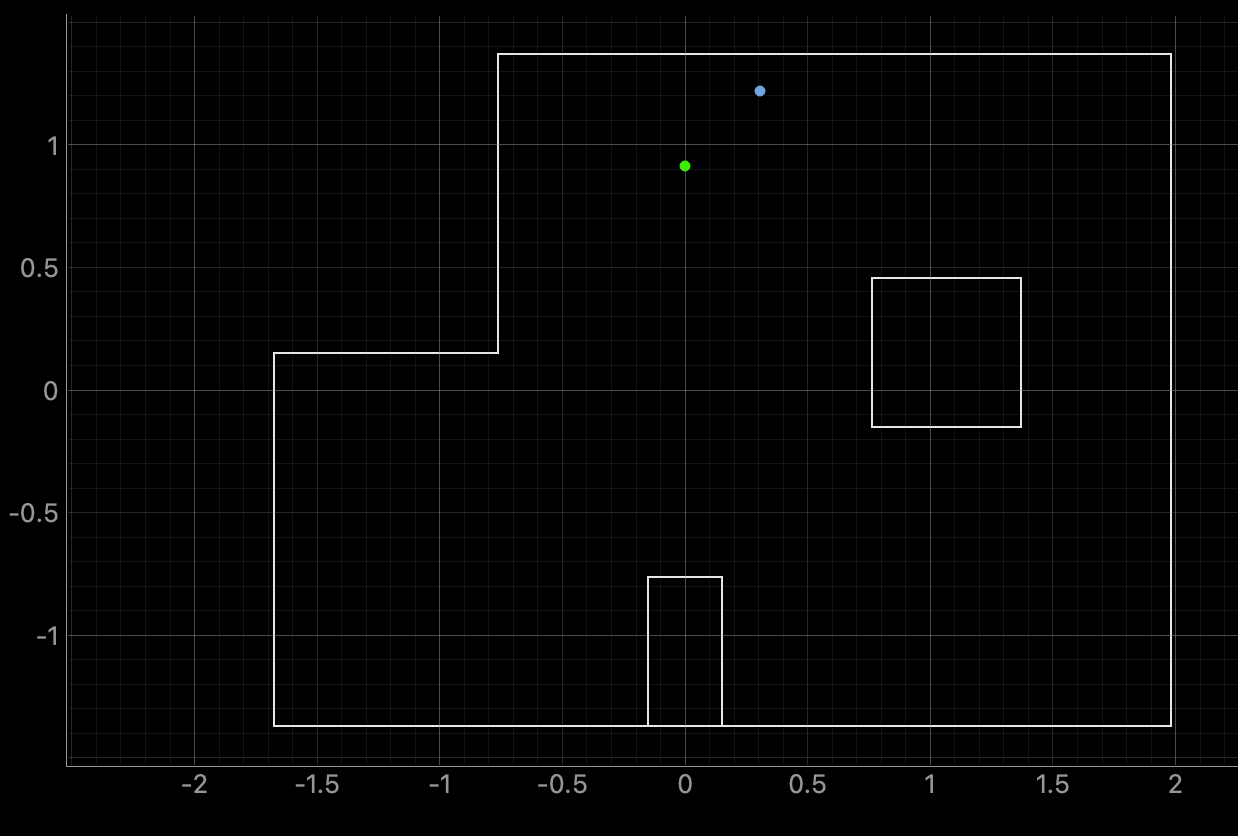
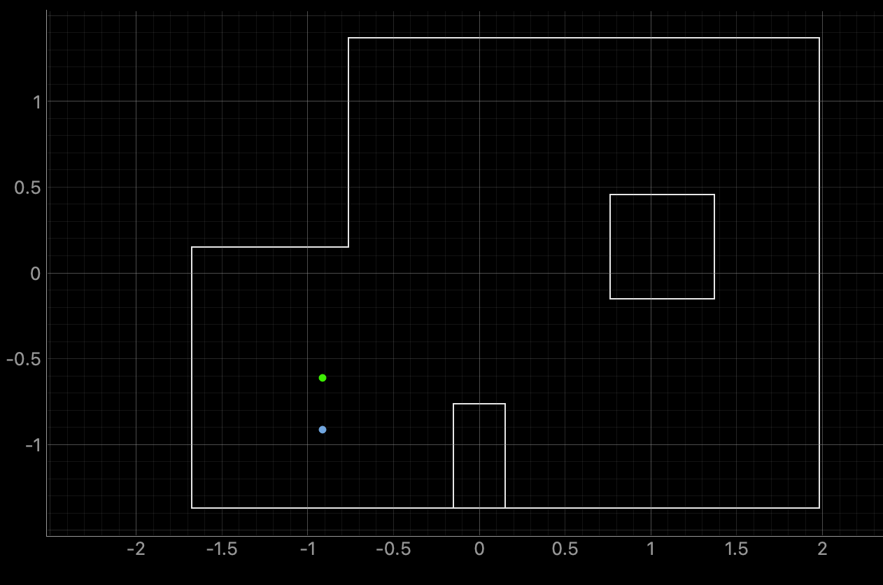
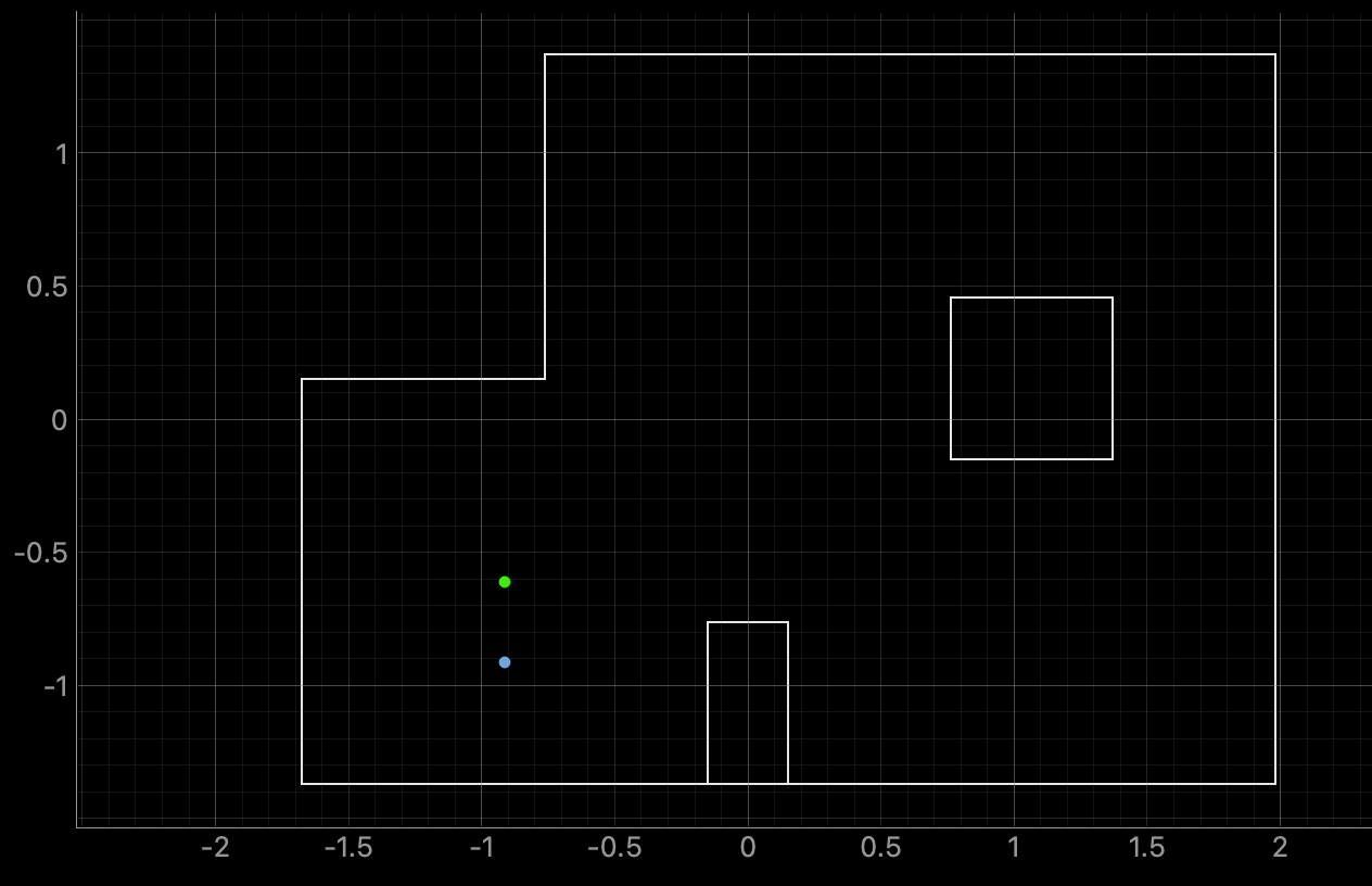
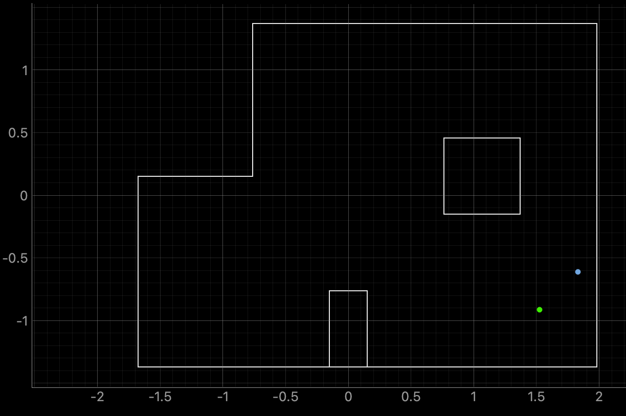
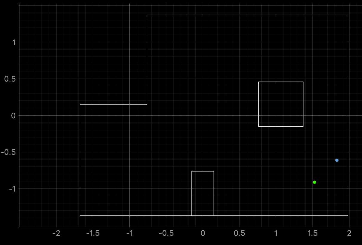
Now I was able to run the Bayes Filter on the real robot in order to localize it. The following graphs represent the result of localizing using a Bayes Filter after collecting 18 data points at each spot, along with the computed probability that the robot exists in that pose.
Spot 1: (0 m, 0.9144 m)
Trial 1:
| True Position | Bayes Localization | Distance from Truth | Reported Probability |
|---|---|---|---|
| (0, 0.9144) | (0.305, 1.219) | 0.431 m | 0.9985 |
Spot 2: (-0.9144 m, -0.6096 m)
Trial 1:
Trial 2:
| True Position | Bayes Localization | Distance from Truth | Reported Probability |
|---|---|---|---|
| (-0.9144, -0.6096) | (-0.914, -0.914) | 0.3044 m | 0.9884 |
Spot 3: (1.524 m, 0.9144 m)
Trial 1:
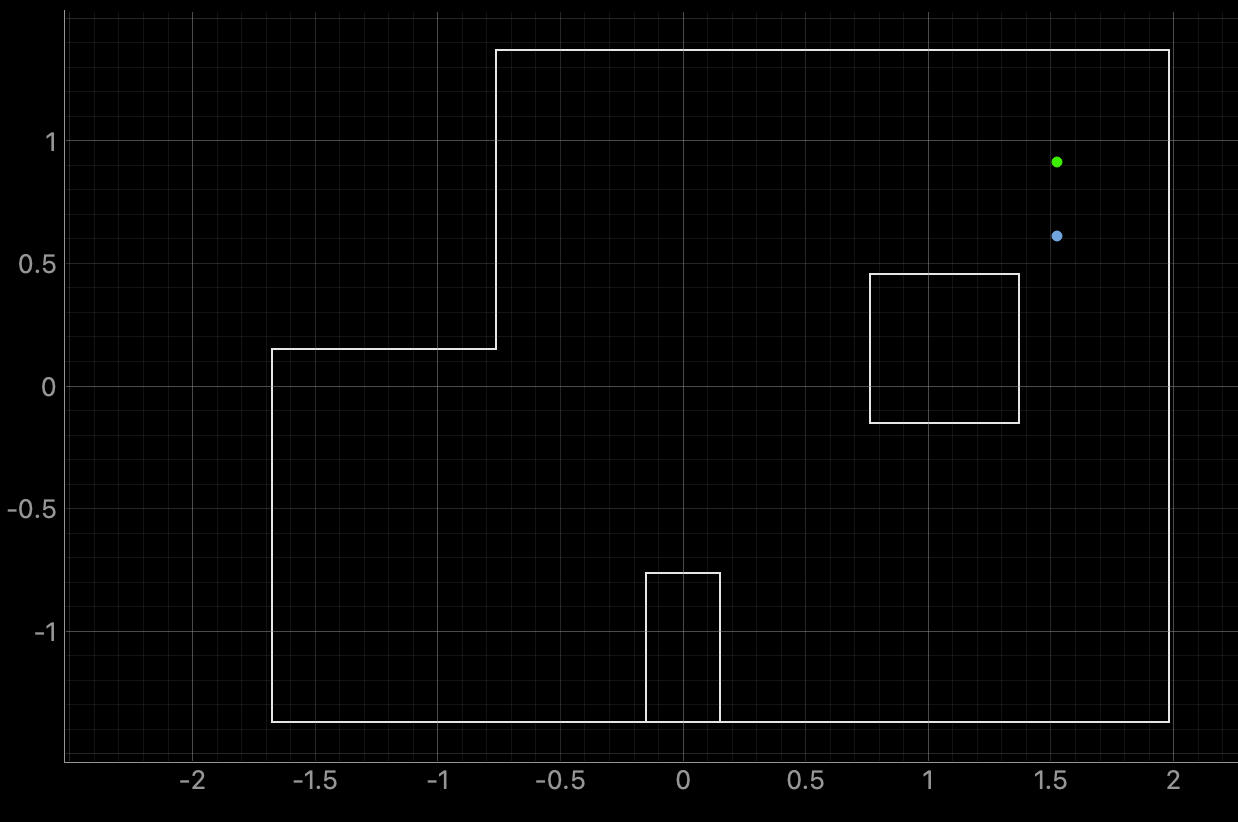
| True Position | Bayes Localization | Distance from Truth | Reported Probability |
|---|---|---|---|
| (1.524, 0.9144) | (1.524,0.610) | 0.3044 m | 0.9999995 |
Trial 2:
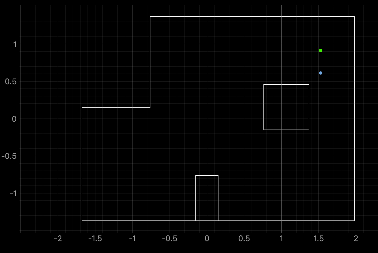
| True Position | Bayes Localization | Distance from Truth | Reported Probability |
|---|---|---|---|
| (1.524, 0.9144) | (1.524,0.610) | 0.3044 m | 0.9999999 |
Spot 4: (0 m, 0 m)
Trial 1:
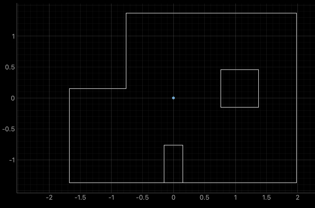
| True Position | Bayes Localization | Distance from Truth | Reported Probability |
|---|---|---|---|
| (0, 0) | (0,0) | 0 m | 1 |
Trial 2:
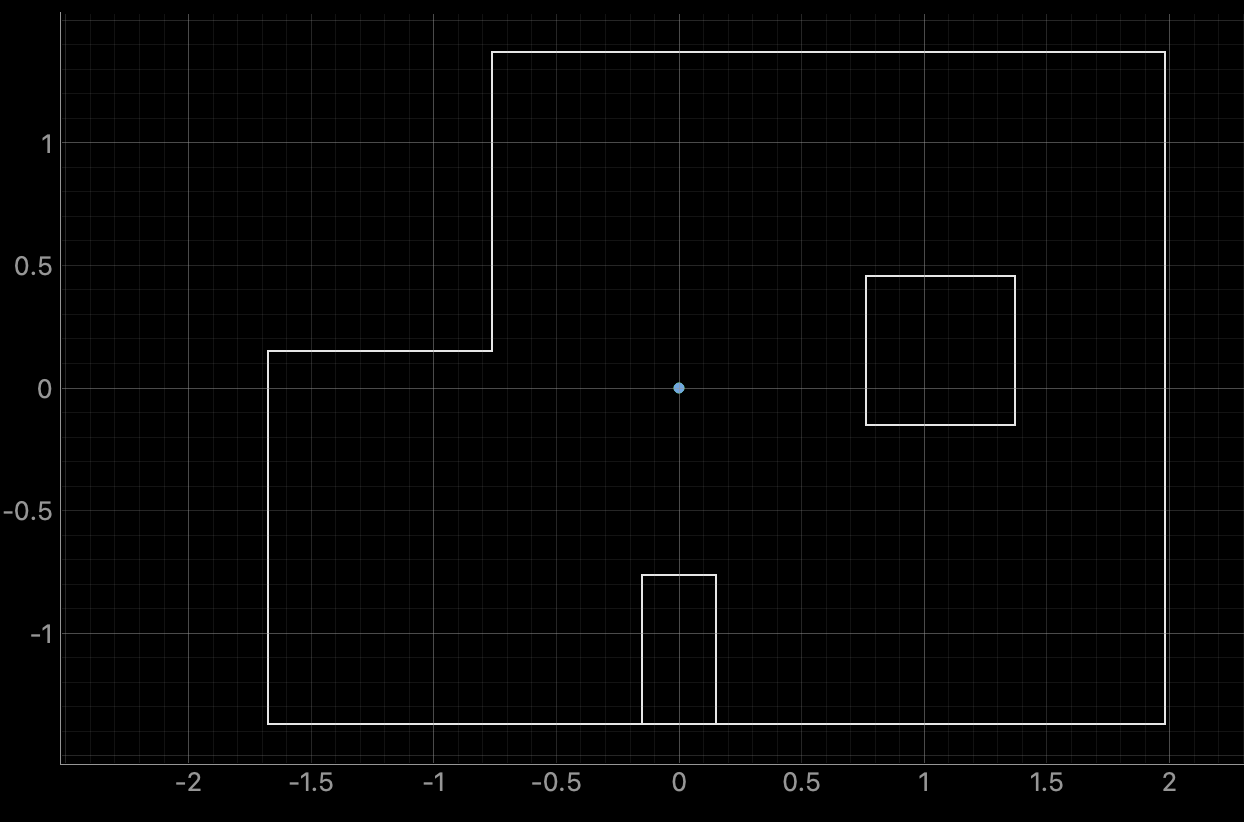
| True Position | Bayes Localization | Distance from Truth | Reported Probability |
|---|---|---|---|
| (0, 0) | (0,0) | 0 m | 0.9999999 |
Spot 5: (1.524 m, -0.9144 m)
Trial 1:
| True Position | Bayes Localization | Distance from Truth | Reported Probability |
|---|---|---|---|
| (1.524, -0.9144) | (1.829,-0.610) | 0.4309 m | 1.0 |
Trial 2:
| True Position | Bayes Localization | Distance from Truth | Reported Probability |
|---|---|---|---|
| (1.524, -0.9144) | (1.829,-0.610) | 0.4309 m | 1.0 |
Bayes Discussion
As it can be seen, the filter did not work perfectly. The localization is most accurate, and pretty confident, at Spot 4, corresponding to the origin of the map. I am assuming that this is because my robot does not achieve zero translation when performing the 360°, and it ends up slightly to the side of where it started. It is possible that this change in position could have less of an effect on the localization at Spot 4 because most of the obstacles are far from that spot, meaning a slight translation in one direction wouldn’t greatly change the measurements. This is not true, however, in corners or next to obstacles because a small robot translation would create a more noticeable change in the measured output. This could also help to explain the large localization errors in these areas of the map.
Additionally, I am concerned about the Bayes Filter reporting probabilities of 1. This value of probability indicates that there is no uncertainty in the estimation. The issue that arises from this can be clearly seen when localizing in Spot 5, where the filter is 100% confident about the robot’s pose, but the filter has output the wrong pose. This means that the filter is 100% in a false state, which is why it is important to avoid having a probability of 1 for any state.
For future iterations, I may ensure that the probability in any state can never be equal to 1 by redistributing a very small amount of probability to other nearby states if this were to happen again.