Lab 10: Grid Localization using Bayes Filter
In this lab, we discretize the robot’s world into multiple grids. We do this in order to better localize in the world. The following image, borrowed from lecture material, can help with visualizing this.
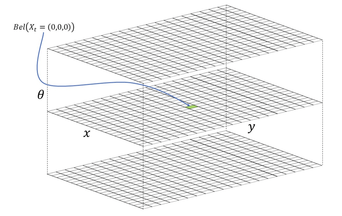
To use these grids, we will implement a Bayes Filter. But first, we need to ensure that the simulation environment in which we are testing the Bayes Filter is functional.
Pre-lab: Using the Simulator
The simulation environment maps the robot’s world and visualizes the robot’s pose. The robot can take distance measurements, and we are able to control both the linear velocity and the radial velocity of the robot.
Open Loop Controller
I first created an open loop controller that made the robot move in a square.
I did this by commanding the robot to move forward, stop moving and turn 90°, and then continuously applying these same commands. The velocity command runs for 1 second, but that is because I force the system to wait 1 second before updating this value. If I had not put this here, I assume that the velocity was constant until it was changed via a new command.
while cmdr.sim_is_running() and cmdr.plotter_is_running():
    cmdr.set_vel(0.5, 0)
    await asyncio.sleep(1)
    cmdr.set_vel(0, 1.5708)
    await asyncio.sleep(1)
    pose, gt_pose = cmdr.get_pose()
    cmdr.plot_odom(pose[0], pose[1])
    cmdr.plot_gt(gt_pose[0], gt_pose[1])
This code resulted in the behavior shown in the video below. The data plotted in red is the raw odometry data, and the data plotted in green is the true position of the robot. The raw odometry data does a terrible job at localizing the robot.
Closed Loop Controller
I created a closed loop controller to perform basic obstacle avoidance on the robot.
minimum_distance_threshold = 0.5
while cmdr.sim_is_running() and cmdr.plotter_is_running():
    sensor_values = cmdr.get_sensor()
    while(sensor_values <= minimum_distance_threshold):
        cmdr.set_vel(0, 1.5708) # turn 10 degrees to the left
        await asyncio.sleep(0.2)
        sensor_values = cmdr.get_sensor()
    cmdr.set_vel(2, 0)
    pose, gt_pose = cmdr.get_pose()
    cmdr.plot_odom(pose[0], pose[1])
    cmdr.plot_gt(gt_pose[0], gt_pose[1])
Whenever the robot was within 0.5 meters of an obstacle directly in front of it, the robot would turn 90° and continue turning until the sensor reported a distance greater than 0.5 meters. Since all of the obstacles within the robot’s world had right corners, a 90° rotation would be sufficient in allowing the robot to avoid most obstacles. Additionally, the robot’s small velocity allowed it to rotate in time before hitting an obstacle. I originally had the robot move at 0.5 m/s, but I noticed that the obstacle avoidance worked just as well when the robot moved at 2 m/s. I don’t believe this result would be replicable in the real world because of the additional momentum of the car.
I noticed that the robot ran into obstacles if they weren’t directly within the line of sight of the robot’s distance sensor. For example, this happens when the sensor’s path of measurement barely misses a close obstacle. The robot then believes that its closest obstacle is much farther away, causing it to run into a wall.
A solution to this could be to have the robot move forward until it is near an obstacle, and then rotate 360° and incrementally take distance measurements. The robot could drive between whichever two angles resulted in consecutive measurements with the largest average distance. Hopefully, this would prevent the robot from running into walls.
Lab: Implementing a Bayes Filter
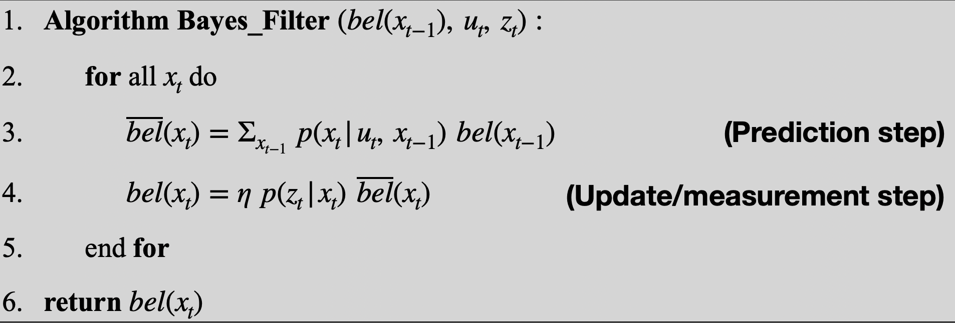
To put it simply, Bayes Filters operate by starting with an initial belief about the state of the robot, and changing the likelihood of this belief in order to better reflect the true state of the robot based on two considerations:
- Given the previous input, and taking into account all possible previous states, what state is the robot likely to find itself in? This is the prediction step of the Bayes Filter.
- Over all possible current states, which states would most likely allow the robot to sense the environment in the way that it had? This is the update step of the Bayes filter.
This algorithm can be visualized below, in an image borrowed from the lecture slides.
Prediction Step
Computing Control
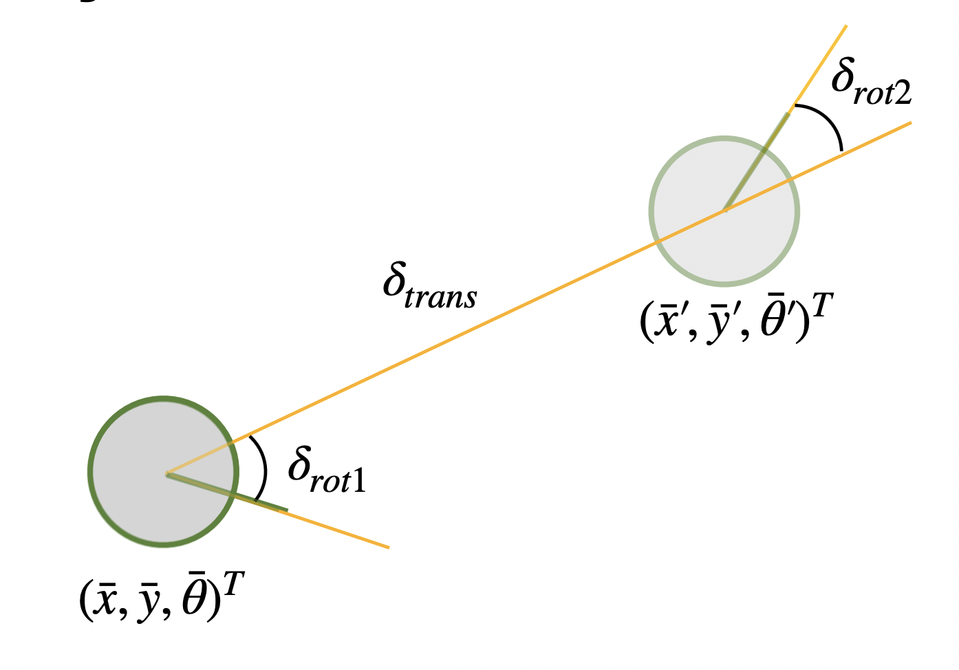
This function took in the current and previous poses to calculate the control input that would move the robot from the previous to current pose.
The control is a combination of an initial rotation, a translation, and a second rotation. A visualization of this can be seen in the image below, which is borrowed from the lecture slides. Here, the robot object associated with x',y',theta' is the current pose, and the robot associated with x,y,theta is the previous pose.
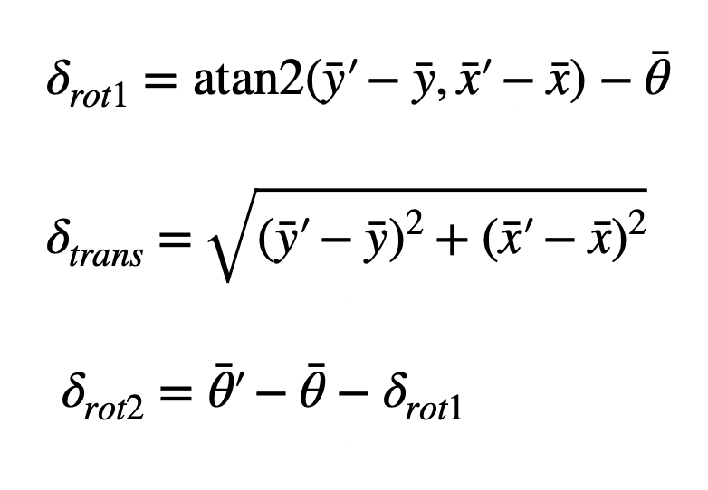
The math behind deriving the two rotations and translation is shown below, also borrowed from the lecture slides.
def compute_control(cur_pose, prev_pose):
    """ Given the current and previous odometry poses, this function extracts
    the control information based on the odometry motion model.
    Args:
        cur_pose  ([Pose]): Current Pose
        prev_pose ([Pose]): Previous Pose
    Returns:
        [delta_rot_1]: Rotation 1  (degrees)
        [delta_trans]: Translation (meters)
        [delta_rot_2]: Rotation 2  (degrees)
    """
    delta_rot_1 = np.degrees(np.atan2(cur_pose[1] - prev_pose[1], cur_pose[0] - prev_pose[0])) - prev_pose[2]
    delta_trans = np.sqrt(((cur_pose[0] - prev_pose[0])**2)+((cur_pose[1] - prev_pose[1])**2))
    delta_rot_2 = cur_pose[2] - prev_pose[2] - delta_rot_1
    return delta_rot_1, delta_trans, delta_rot_2
Odometry Motion Model
This function returns the probability that the robot moved from a previous pose to the current pose when given an ideal control input u. We use compute_control() in order to determine what the robot actually did to move between the poses, and compared this movement to what it would have done if it had followed u from the previous pose.
We assume that the actual control inputs differ from the ideal control input following a normal distribution, and we use this to determine the probability that the robot could move from the previous pose to the current one given input u.
def odom_motion_model(cur_pose, prev_pose, u):
    """ Odometry Motion Model
    Args:
        cur_pose  ([Pose]): Current Pose
        prev_pose ([Pose]): Previous Pose
        (rot1, trans, rot2) (float, float, float): A tuple with control data in the format
                                                   format (rot1, trans, rot2) with units (degrees, meters, degrees)
    Returns:
        prob [float]: Probability p(x'|x, u)
    """
    delta_rot_1, delta_trans, delta_rot_2 = compute_control(cur_pose, prev_pose)
    delta_rot_1 = mapper.normalize_angle(delta_rot_1)
    delta_rot_2 = mapper.normalize_angle(delta_rot_2)
    ideal_rot_1, ideal_trans, ideal_rot_2 = u
    ideal_rot_1 = mapper.normalize_angle(ideal_rot_1)
    ideal_rot_2 = mapper.normalize_angle(ideal_rot_2)
    prob = loc.gaussian(delta_rot_1, ideal_rot_1, loc.odom_rot_sigma)*loc.gaussian(delta_rot_2, ideal_rot_2, loc.odom_rot_sigma)*loc.gaussian(delta_trans, ideal_trans, loc.odom_trans_sigma)
    return prob
Motion Model Based Prediction
The prediction step of the Bayes Filter is almost finished. The only thing left is to iterate over all possible previous states and current states, and use the known input and previous beliefs about the states to make a prediction on where the state has moved.
def prediction_step(cur_odom, prev_odom):
    """ Prediction step of the Bayes Filter.
    Update the probabilities in loc.bel_bar based on loc.bel from the previous time step and the odometry motion model.
    Args:
        cur_odom  ([Pose]): Current Pose
        prev_odom ([Pose]): Previous Pose
    """
    current_input = compute_control(cur_odom, prev_odom)
    loc.bel_bar = np.zeros((mapper.MAX_CELLS_X, mapper.MAX_CELLS_Y, mapper.MAX_CELLS_A))
    for i in range((mapper.MAX_CELLS_X)):
        for j in range((mapper.MAX_CELLS_Y)):
            for k in range((mapper.MAX_CELLS_A)):
                if loc.bel[i,j,k] >= 0.0001:
                    for x in range((mapper.MAX_CELLS_X)):
                        for y in range((mapper.MAX_CELLS_Y)):
                            for a in range((mapper.MAX_CELLS_A)):
                                loc.bel_bar = loc.bel_bar + odom_motion_model(mapper.from_map(x, y, a), mapper.from_map(i, j, k), current_input)*loc.bel[i,j,k]
    loc.bel_bar = loc.bel_bar/np.sum(loc.bel_bar)
Update Step
Sensor Model Implementation
The sensor_model() function takes in the measurement data gathered by the robot about its current pose. The robot collected this data by spinning in place and taking a distance measurement every 20°. It was assumed that the measured data would belong to a normal distribution of possible readings centered about the true distance value, and this was used in order to associate a probability with each measurement.
def sensor_model(obs):
    """ This is the equivalent of p(z|x).
    Args:
        obs ([ndarray]): A 1D array consisting of the true observations for a specific robot pose in the map
    Returns:
        [ndarray]: Returns a 1D array of size 18 (=loc.OBS_PER_CELL) with the likelihoods of each individual sensor measurement
    """
    prob_array = []
    for i in range(mapper.OBS_PER_CELL):
        prob_array.append(loc.gaussian(loc.obs_range_data[i], obs[i], loc.sensor_sigma))
    prob_array = np.array(prob_array)
    return prob_array
Update Step
To finish the update step, it is necessary to iterate over all possible current states, determine the likelihood of seeing distance data similar to what the robot recorded at any given current state, and use this in combination with the predicted beliefs to improve the certainty of the belief of the robot.
def update_step():
    """ Update step of the Bayes Filter.
    Update the probabilities in loc.bel based on loc.bel_bar and the sensor model.
    """
    loc.bel = np.zeros((mapper.MAX_CELLS_X, mapper.MAX_CELLS_Y, mapper.MAX_CELLS_A))
    for i in range((mapper.MAX_CELLS_X)):
        for j in range((mapper.MAX_CELLS_Y)):
            for k in range((mapper.MAX_CELLS_A)):
                probs = sensor_model(mapper.get_views(i, j, k))
                total_prob = 1
                for n in range(len(probs)):
                    total_prob = total_prob*probs[n][0]
                loc.bel[i,j,k] = total_prob*loc.bel_bar[i,j,k]
    loc.bel = loc.bel/np.sum(loc.bel)
Results of the Simulation
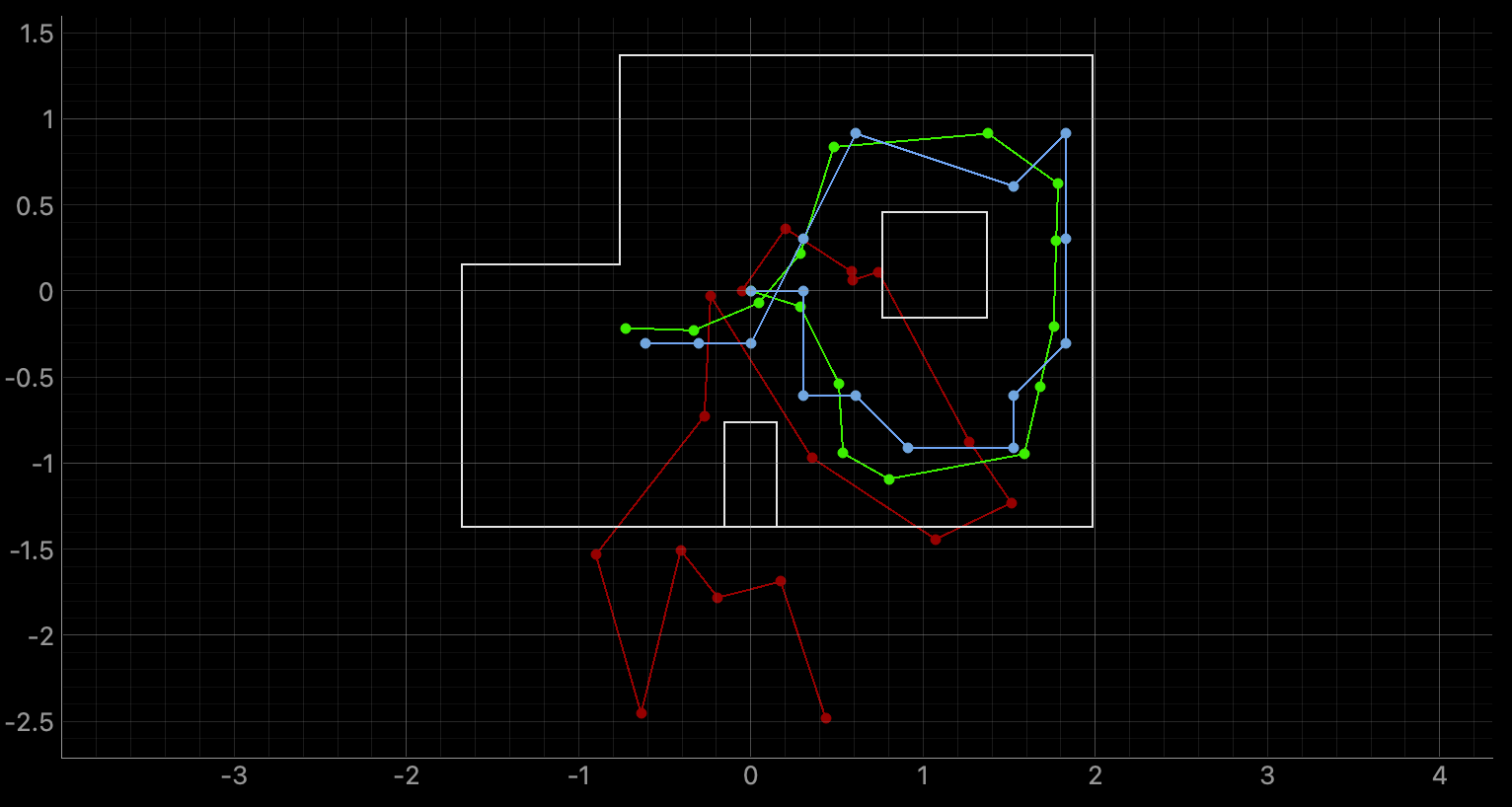
After implementing the Bayes Filter, the robot was able to localize significantly better. In the image below, the green dots and lines represent the true position of the robot, while the blue and red represent the belief output from the Bayes Filter and the dead reckoning output, respectively. It is incredibly clear how terrible the data in red tracks the location of the car in its environment, even having it drive through walls.
The output of the Baye Filter, however, much more closely approaches the true position of the robot.
Acknowledgements
I referenced Stephan Wagner’s and Tyler Wisniewski’s previous work in order to double check mine.